QA0003

MATLAB script with notes in HTML format:

Q: How to detect tinted cells in input image, and then calculate each perimeter and centroid of detected cell.

A:

Part I - Prepare input image ............................................................................................... 1

Part II - Attempt with kmeans ............................................................................................ 9

Part III - bwboundaries ........................................................................................................ 11

Image 'clean-up' tools that may be useful ............................................................ 13

Part IV Centroids ................................................................................................................. 21

Problem with call to regionprops to get area of each cell .............................. 21

Part V suggested further work ........................................................................................ 24

Part VI Area .......................................................................................................................... 26

% catch_tilted_cells.m
%
% short description: % image segmentation: catch high pigmentation cells with
% histogram and bwboundaries, without kmeans.

% Script Author: John Bofarull Guix, jgb2012@sky.com
%
%
% Given the input image supplied by the question originator, this script obtains
% coordinates of only the cells of interest tilted in saturated magenta, draws
% perimeter, and calculates centroids, while applying a numeral to each cell
%
% The area of each cell may also be of interest, yet it has not been asked.
% The question originator repeatedly mentioned kmeans, but the standard kmeans
% requires of knowledge, if only approximate, of the amount of clusters, otherwise
% in a case like the input image, the amount of sought cells my range from non, just
% a few, or perhaps several hundreds, or even higher orders of magnitude.
%
% applying Mathworks examples:
% 1.- Detecting a Cell Using Image Segmentation
% 2.- https://uk.mathworks.com/help/images/identifying-round-objects.html

close all;clear all;clc

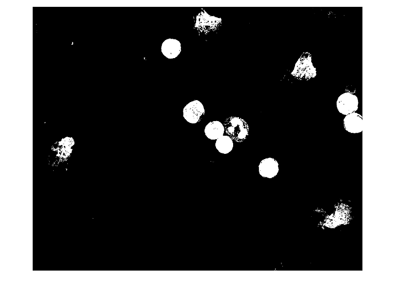
Part I - prepare input image

display and measure input image

A=imread('001.jpg');
hf1=figure(1);imshow(A);ax1=gca

Ar=A(:,:,1);Ag=A(:,:,2);Ab=A(:,:,3);
[sz1,sz2]=size(Ar);

Warning: Image is too big to fit on screen; displaying at
50%
ax1 =
Axes with properties:

XLim: [0.500000000000000 1.712500000000000e+03]
YLim: [0.500000000000000 1.368500000000000e+03]
XScale: 'linear'
YScale: 'linear'
GridLineStyle: '-'
Position: [1×4 double]
Units: 'normalized'

Use GET to show all properties

command imsegkmeans is probably what you are looking for, but you need to have the upgraded image processing toolbox, that comes with MATLAB version R2019. Try installing MATLAB R2019 student version and then use imsegkmeans. imsegkmeans is not a public function.

B=rgb2lab(A); figure;imshow(B); B2=B(:,:,2:3); B2 = im2single(B2); nColors = 3;

% repeat the clustering 3 times to avoid local minima

pixel_labels = imsegkmeans(B2,nColors,'NumAttempts',3);

the cells of interest are all distinctively marked with saturated magenta colour. So up for magenta that in this picture all magenta pixels have approximately proportion value around [.5 0 1]

Amag=Ar+Ab;

measuring range of magenta pixels

maxAmag=double(max(max(Amag)))
minAmag=double(min(min(Amag)))

% Amag2=255/maxAmag*(Amag-minAmag); % manual adjustment, not needed
% Amag1=double(Amag(:,:,1));

maxAmag =
255
minAmag =
89

the cells of interest are holes, let's turn them into peaks: inverting pixel values

Amag2=double(maxAmag-Amag);
maxAmag2=max(max(Amag2))
minAmag2=min(min(Amag2))

maxAmag2 =
166
minAmag2 =
0

stretching image to use all available range [0 255]

Amag3=uint8(255/maxAmag2*Amag2);
hf3=figure(2);imshow(Amag3);ax2=gca;

Warning: Image is too big to fit on screen; displaying at
50%

One can manually adjust contrast: the output has to be saved through the File menu of the figure window,

figure(3);imcontrast(hf3)

% or input grey scale thresholds directly into imadjust.
A4=imadjust(Amag3,[.1921 ; .2274],[]);
figure(4);imshow(A4);ax4=gca

Warning: Image is too big to fit on screen; displaying at
50%
ax4 =
Axes with properties:

XLim: [0.500000000000000 1.712500000000000e+03]
YLim: [0.500000000000000 1.368500000000000e+03]
XScale: 'linear'
YScale: 'linear'
GridLineStyle: '-'
Position: [1×4 double]
Units: 'normalized'

Use GET to show all properties

2D Laplacian

LA1=del2(double(A4));
% LA1=del2(double(A4(:,:,1)));LA2=del2(double(A4(:,:,2)));LA3=del2(double(A4(:,:,3)));
figure(5);imshow(LA1)

[szla1 szla2]=size(LA1)

min(min(LA1))
max(max(LA1))

LA1(LA1<0)=0;
LA1(LA1>=1)=1;

figure(6);imshow(LA1);ax6=gca % check it looks the same

min(min(LA1)) % now LA1 pixels only range between [0 1]
max(max(LA1))

n1=find(LA1==1);
[nx ny]=ind2sub([szla1 szla2],n1);

% therefore I am not using del2 again, but [nx ny] are use in the first histogram
% just as alternative to kmeans without a reasonable guess or wherabouts of the
% amount of cells to catch, which is precisely part of the sought answer.

Warning: Image is too big to fit on screen; displaying at
50%
szla1 =
   1368
szla2 =
   1712
ans =
-255
ans =
255
Warning: Image is too big to fit on screen; displaying at
50%
ax6 =
Axes with properties:

XLim: [0.500000000000000 1.712500000000000e+03]
YLim: [0.500000000000000 1.368500000000000e+03]
XScale: 'linear'
YScale: 'linear'
   GridLineStyle: '-'
Position: [1×4 double]
   Units: 'normalized'

Use GET to show all properties
ans =
0
ans =
1

Part II - attempt with kmeans

Checking the obtained pixel locations [nx ny] correspond to cell skins once you know the coordinates of the cell skins you can calculate each cell centroid.

hold(ax6,'on')
plot(ax6,ny,nx,'ro')

% note that to correctly plot ny goes ahead of nx

% lining up point coordinates
X=[nx ny];

% Let's assume that there may be around, approximately, 30 cells
[idx,sumd,CD]=kmeans(X,3);

% idx vector contains predicted clustersr

x1 = min(X(:,1)):0.01:max(X(:,1));
x2 = min(X(:,2)):0.01:max(X(:,2));
% [x1G,x2G] = meshgrid(x1,x2);
% XGrid = [x1G(:),x2G(:)]; % Defines a fine grid on the plot

% problem:
% idx2Region = kmeans(XGrid,3,'MaxIter',1,'Start',CD);
   % While attempting to assign each node in the grid to the closest centroid
   % kmeans call the output of meshgrid, that for exercise is already of
   % size above 1x150000. This itself is not a problem, but since meshgrid
   % calls repmat, such large values for a student version saturates memory
   % forcin the following error:
% Error using repmat
% Requested 170401x136701 (173.6GB) array
% exceeds maximum array size preference.
% Creation of arrays greater than this limit
% may take a long time and cause MATLAB to
% become unresponsive. See array size limit
% or preference panel for more information.
% Error in meshgrid (line 58)
% xx = repmat(xrow,size(ycol));
%
% and I am mentioning again, the second field input to kmeans is a guess
% of the amount of cells to look for. One can interate kmeans to sweep that guess
% and then have the user inspecting for coherence, but in my opinion,
% perhaps there's a combination of input parameters that simplify such obstacle,
% but on 1st approach, kmeans is not as robust as simply processing the boundaries
% obtained with bwboundaries.

% for instance, let's run 2 histograms, one for each x y boundary coordinates
% nx ny have been obtained with del2, but are quite the same points that are going
% to be obtained in next point with bwboundaries.

figure(7);histogram(nx,floor(numel(nx)/12))
figure(8);histogram(ny,floor(numel(ny)/12))

% histogram too wide to catch the cells of interest, yet one can readily observe that
% there's correlation between histogram peaks and amount of cells, as well as cell locations.

Part III - bwboundaries

back to A4 using command bwboundaries obtains the coordinates of cell skins in variable B.

[B,L] = bwboundaries(A4,'noholes');
hold(ax4,'on')
for k = 1:length(B)
boundary = B{k};
plot(ax4,boundary(:,2),boundary(:,1),'r','LineWidth',2)
end

L1=[]
for k=1:1:size(B,1)
L1=[L1 size(B{k},1)];
end

length(L1) % 577 way too many too small cells taken as valid cells.

figure(9);histogram(L1,length(L1));grid on
title('histogram red tag cells boundary lengths')

% histogram seems apparently void above bin 50, but in fact the cells of interest
% created amplitude 1 peaks, one needs to zoom in, at the exact.

L1 =
[]
ans =
577

Image 'clean-up' tools that may be useful

one may or may not use the following, but I mention it because the input image is usually unknown a these corrections, along many others mentioned in the Image Processing MATLAB online and local help pages

Inflating white pixels with strel line.

npx=5
se90 = strel('line', npx, 90);
se0 = strel('line', npx, 0);
r0=4
ser=strel('disk',r0)
A5 = imdilate(A4, [se90 se0]);
figure(10);imshow(A5), title('filling holes wth dilated gradient mask');

npx =
5
r0 =
4
ser =
strel is a disk shaped structuring element with properties:

Neighborhood: [7×7 logical]
Dimensionality: 2
Warning: Image is too big to fit on screen; displaying at
50%

Attempting a bit of fill-up before applying bwboundaries, now strel diamond.

for k=1:1:10
seD = strel('diamond',1);
A6 = imerode(A5,seD);
A6 = imerode(A6,seD);
end
figure(11);imshow(A6); title('filing edgees');

A62 = imclearborder(A6, 4);
figure(12); imshow(A62); ax12=gca; title('cleared border image');

Warning: Image is too big to fit on screen; displaying at
50%
Warning: Image is too big to fit on screen; displaying at
50%

manually removing 'small' false cells and counting cells of interest with histogram.

again detecting boundaries

[B2,L2] = bwboundaries(A62,'noholes');
hold(ax12,'on')
for k = 1:length(B2)
boundary2 = B2{k};
plot(ax12,boundary2(:,2),boundary2(:,1),'r','LineWidth',2)
end

L2=[];
for k=1:1:size(B2,1)
L2=[L2 size(B2{k},1)];
end

length(L2)

% apparently there are 119 cells, but the majority of these hits are too small to be
% considered cells, let's eliminate all too-small false cells.
%

% no cell has as many as 1050 pixels along respective perimeter.
% All cell perimeters are shorter than 1050, so setting histogram bin width to 1
% and the amount of histogram bins to 1050.
upper_limit_cell_perimeter=1050

figure(14);hst1=histogram(L2,upper_limit_cell_perimeter)

% central value of each bin
nL0=ceil(cumsum(diff(hst1.BinEdges)));

% histogram count for each bin

L0=hst1.Values;

% Now with figure marker manually measure diameter of any red contour cell.
% Its about 110 pixels so any cell perimeter is about 220 pixels long, roughly.

lower_limit_cell_perimeter=150

% To find out how many counts above lower_limit_cell_perimeter
% one could use
% [vh,nh]=find(hst1.BinEdges>150)
%
% but because histogram bins are arranged as consecutive increasing numerals, then
% instead one can use

nL_1=nL0(nL0>lower_limit_cell_perimeter);

% how many cells for each possible perimeter length
L_1=L0(nL_1);
L_1(L_1>0);

% it turns out that there's only one cell for each perimeter value, but it could be
% the case that many cells have exactly same perimeter length

% perimeter lengths are
P=nonzeros(nL_1.*L_1)

% As mentioned, if one or more bins above lower_limit_cell_perimeter show values >1
% then use the following for loop to obtain in one variable all perimeter lengths from cells of interest
P1=[]
for k=1:1:length(L_1)
P1=[P1;repmat(nL_1(k),L_1(k),1)];
end
P1==P

LB=[]
for k=1:1:length(B)
   L21=length(B{k});
   LB=[LB length(B{k})];
end

% indices pointing at those boundaries in B longer than lower_limit_cell_perimeter
nLB=find(LB>lower_limit_cell_perimeter)

% B2 contains the coordinates of long boundaries
B3={}
for k=1:1:numel(nLB)
   B3=[B3 B{nLB(k)}];
end

% copying boundaries B3 on high contrast image
hold(ax2,'on')
for k = 1:length(B3)
boundary3 = B3{k};
plot(ax2,boundary3(:,2),boundary3(:,1),'r','LineWidth',5)
end

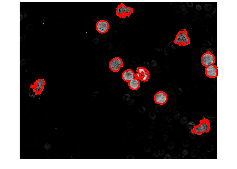
% copying boundaries B3 of intereset on input signal
hf10=figure(10);imshow(A);ax10=gca
hold(ax10,'on')
for k = 1:length(B3)
boundary3 = B3{k};
plot(ax10,boundary3(:,2),boundary3(:,1),'r','LineWidth',5)
end

ans =
119
upper_limit_cell_perimeter =
   1050
hst1 =
Histogram with properties:

Data: [1×119 double]
Values: [1×1050 double]
   NumBins: 1050
BinEdges: [1×1051 double]
BinWidth: 0.975500000000000
   BinLimits: [1.800000000000000 1.026075000000000e+03]
   Normalization: 'count'
   FaceColor: 'auto'
   EdgeColor: [0 0 0]

Use GET to show all properties
lower_limit_cell_perimeter =
150
P =
162
309
322
368
495
630
641
702
P1 =
[]
ans =
8×1 logical array
1
1
1
1
1
1
1
1
LB =
[]
nLB =
   21 113 116 126 151 217 270 303 379 468
B3 =
0×0 empty cell array
Warning: Image is too big to fit on screen; displaying at
50%
ax10 =
Axes with properties:

XLim: [0.500000000000000 1.712500000000000e+03]
YLim: [0.500000000000000 1.368500000000000e+03]
XScale: 'linear'
YScale: 'linear'
   GridLineStyle: '-'
Position: [1×4 double]
   Units: 'normalized'

Use GET to show all properties

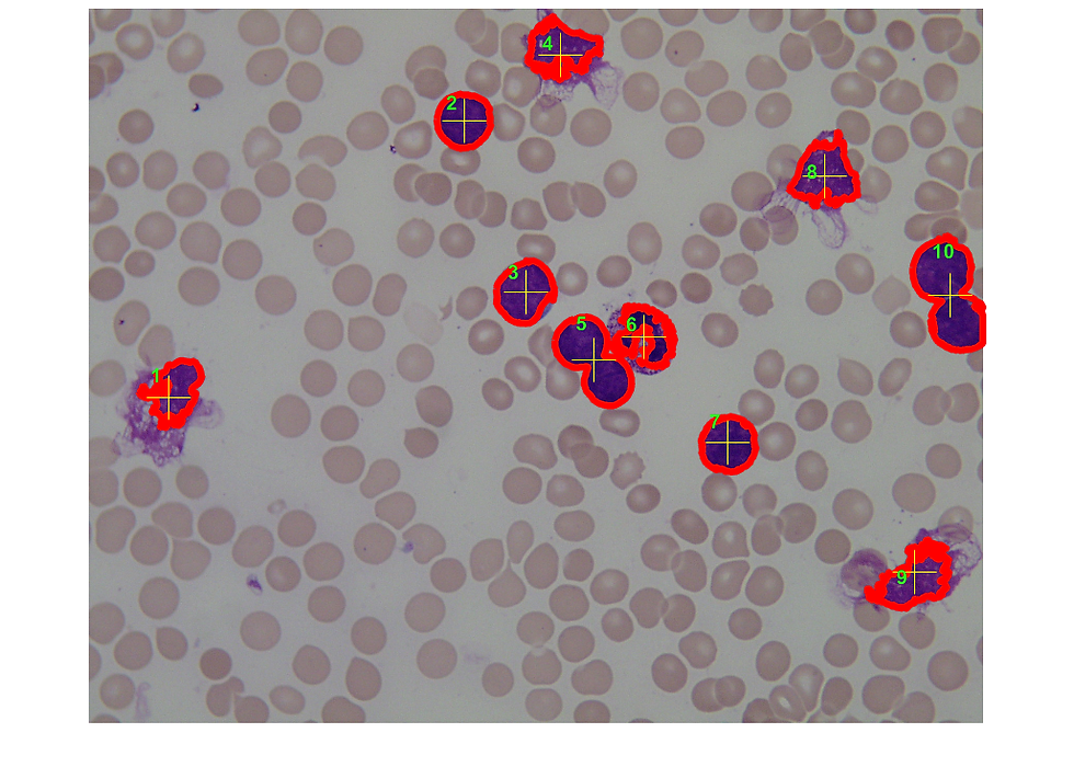
Part IV - Centroids

There's a problem when calling regionprops to get cell areas

either

stats = regionprops(L2,'Area','Centroid')
% or
% stats = regionprops(L2,'Centroid')
length(stats)

% regionprops is applied to the image before using histogram to exactly obtain the
% cells of interest. Either clean enough image has been produced to then apply
% regionprops, or in this exerrcise, once the clean is obtained, using regionprops
% would force to rebuild an image with solid cells and then apply regionprops
% to avoid excessive regrowth when applying regionprops, that in turn applies
% bwboundary, on the already obtained boundaries,

hf11=figure(11);imshow(A);ax11=gca
hold(ax11,'on')

for k = 1:length(B3)

boundary = B3{k};
delta_sq = diff(boundary).^2;      % cell k simplified perimeter length in pixels
p4 = sum(sqrt(sum(delta_sq,2)));

area = stats(k).Area; % cell k area of cell k

metric = 4*pi*area/p4^2;    % cell k roundness

metric_string = sprintf('%2.2f',metric); % display results in command window.

% if metric > threshold    % mark objects above the threshold with red circle
centroid = stats(k).Centroid;
   plot(ax11,centroid(1),centroid(2),'ro');
% end

text(ax11,boundary(1,2)-35,boundary(1,1)+13,metric_string,'Color','y','FontSize',14,'FontWeight','bold')

end

% therefore the figures produced belong to one of the many too small cells, the
% numbers of interest being cluttered.
% In any case there's no need to sweep through all cells in the half way image
% with many 'too small' cells when one aready has B3.

stats =
1026×1 struct array with fields:
   Area
   Centroid
ans =
   1026
Warning: Image is too big to fit on screen; displaying at
50%
ax11 =
Axes with properties:

XLim: [0.500000000000000 1.712500000000000e+03]
YLim: [0.500000000000000 1.368500000000000e+03]
XScale: 'linear'
YScale: 'linear'
GridLineStyle: '-'
Position: [1×4 double]
   Units: 'normalized'

use GET to show all properties

fixing meaningless result when attempting to apply last for loop of example

https://uk.mathworks.com/help/images/identifying-round-objects.html

% and bwarea cannot be applied without again spending time building solid cells,
% that for the case, such point has not been asked, therefore the area calculation is omitted.

% close(hf1)

hf20=figure(20);imshow(A);ax20=gca
hold(ax20,'on')

for k = 1:length(B3)
boundary3 = B3{k};
plot(ax20,boundary3(:,2),boundary3(:,1),'r','LineWidth',5)
end

for k = 1:length(B3)

boundary = B3{k};
centroid_1=1/size(boundary,1)*sum(boundary(:,1));
centroid_2=1/size(boundary,1)*sum(boundary(:,2));
centroid=floor([centroid_1 centroid_2])

plot(ax20,centroid(2),centroid(1),'+y','MarkerSize',31);

text(ax20,centroid(2)-35,boundary(1)-35,num2str(k),'Color','g','FontSize',14,'FontWeight','bold')

end

Warning: Image is too big to fit on screen; displaying at
50%
ax20 =
Axes with properties:

XLim: [0.500000000000000 1.712500000000000e+03]
YLim: [0.500000000000000 1.368500000000000e+03]
XScale: 'linear'
YScale: 'linear'
   GridLineStyle: '-'
Position: [1×4 double]
   Units: 'normalized'

Use GET to show all properties
centroid =
746 154
centroid =
215 719
centroid =
544 838
centroid =
   89 904
centroid =
674 967
centroid =
629    1064
centroid =
832    1224
centroid =
322    1410
centroid =
   1080    1581
centroid =
550    1649

Part V - suggested further work

6.1.- cells 5 and 10 are obviously 2 cells each. It's just that both have isthmi broad enough to confuse bwboundaries.

% bare
% [centers, radii, metric] = imfindcircles(A4,[90 140])
% doesn't catch anything no matter what radii values input.

% but setting object polarity to dark, the detection of all round
% heads is immediate

Rmin=40;Rmax=150
[centersBright, radiiBright] = imfindcircles(A,[Rmin Rmax],'ObjectPolarity','bright');
[centersDark, radiiDark] = imfindcircles(A,[Rmin Rmax],'ObjectPolarity','dark');

hf40=figure(40);imshow(A);ax40=gca
hold(ax40,'on')
viscircles(centersDark, radiiDark,'EdgeColor','y');

% no attempt will be made to catch the cells that do not look like circles with
% imfindcircles.

Rmax =
150
Warning: You just called IMFINDCIRCLES with a large
radius range. Large radius ranges reduce algorithm
accuracy and increase computational time. For high
accuracy, relatively small radius range should be used. A
good rule of thumb is to choose the radius range such
that Rmax < 3*Rmin and (Rmax - Rmin) < 100. If you have a
large radius range, say [20 100], consider breaking it up
into multiple sets and call IMFINDCIRCLES for each set
separately, like this:

[CENTERS1, RADII1, METRIC1] = IMFINDCIRCLES(A, [20 60]);
[CENTERS2, RADII2, METRIC2] = IMFINDCIRCLES(A, [61 100]);

Warning: You just called IMFINDCIRCLES with a large
radius range. Large radius ranges reduce algorithm
accuracy and increase computational time. For high
accuracy, relatively small radius range should be used. A
good rule of thumb is to choose the radius range such
that Rmax < 3*Rmin and (Rmax - Rmin) < 100. If you have a
large radius range, say [20 100], consider breaking it up
into multiple sets and call IMFINDCIRCLES for each set
separately, like this:

[CENTERS1, RADII1, METRIC1] = IMFINDCIRCLES(A, [20 60]);
[CENTERS2, RADII2, METRIC2] = IMFINDCIRCLES(A, [61 100]);

Warning: Image is too big to fit on screen; displaying at
50%

ax40 =
Axes with properties:

XLim: [0.500000000000000 1.712500000000000e+03]
YLim: [0.500000000000000 1.368500000000000e+03]
XScale: 'linear'
YScale: 'linear'
GridLineStyle: '-'
Position: [1×4 double]
Units: 'normalized'

Use GET to show all properties

Catching the roundheads: