example 10.4

ZIP with MATLAB scripts and note:

example 10.4 notes:

Obtaining Vip3(a1,a3) - Symbolic approach

As in [POZAR] pg514 one can reach the sought symbolic expression IP3(a1,a3) with the symbolic toolbox:

syms w1 w2 y V0

syms a1 a2 a3

y=a1*V0*(cos(w1)+cos(w2))+ ...

a2*V0^2*(cos(w1)+cos(w2))^2+ ...

a3*V0^3*(cos(w1)+cos(w2))^3

y2=combine(expand(y),'sincos')

Pw1=.5*a1^2*V0^2

P_2w1_w2=.5*(3*V0^3*a3/4)^2

eq1=.5*a1^2*V0^2==.5*(3*V0^3*a3/4)^2

Vip3=solve(eq1,V0)

y2 =

V0^2*a2 + V0^2*a2*cos(w1 + w2) + (9*V0^3*a3*cos(w1))/4 + (9*V0^3*a3*cos(w2))/4 + V0^2*a2*cos(w1 - w2) + (3*V0^3*a3*cos(w1 - 2*w2))/4 + (3*V0^3*a3*cos(w1 + 2*w2))/4 + (3*V0^3*a3*cos(2*w1 + w2))/4 + (V0^2*a2*cos(2*w1))/2 + (V0^2*a2*cos(2*w2))/2 + (V0^3*a3*cos(3*w1))/4 + (V0^3*a3*cos(3*w2))/4 + (3*V0^3*a3*cos(2*w1 - w2))/4 + V0*a1*cos(w1) + V0*a1*cos(w2)

Vip3 =

0

-(16*(-(3*a1*a3)/64)^(1/2))/(3*a3)

(16*(-(3*a1*a3)/64)^(1/2))/(3*a3)

-(16*((3*a1*a3)/64)^(1/2))/(3*a3)

(16*((3*a1*a3)/64)^(1/2))/(3*a3)

Since it's just a single value, with sign change, the expression matches [POZAR] pg516.

Vip3=Vip3(Vip3~=0);

Vip3=Vip3(end)

IIP3=.5*Vip3^2

OIP3=.5*a1^2*Vip3^2

Vip3 =

(16*((3*a1*a3)/64)^(1/2))/(3*a3)

IIP3 =

(2*a1)/(3*a3)

OIP3 =

(2*a1^3)/(3*a3)

General Expression of Linear Intermodulation Products

Given a set of input frequencies f and a roof amount N for highest single carrier intermodulation in to be considered,

N=3 % linear intermod order roof for a single carrier

f=[1.5 2.1 3.8 5.3 5.4]; % [GHz]

Such set f of non-coherent input carriers can be combined potentially obtaining as many output harmonics with the following expression:

± n(1)*f(1) ± n(2)*f(2) .. ± n(N)*f(N)

The total amount of potential spurs is

size(combinator(N,numel(f),'p','r'),1)* ... % all positive

size(combinator(2,numel(f),'p','r'),1) % adding sign combinations

=

7776

When considering single carrier N-th Order intercept point calculations, regardless the total amount of carriers, for instance in advance of a measurement, one has to decide how many harmonics to be taken into account by choosing N in advance of calculations.

In general signal phases could be taken into account, but because distortion measurements are saturation tests usually out of operating margin, one goes straight to worst case scenario, were all interferers or test tones are in phase.

Intermodulation products are often simply referred as spurs.

If for instance, here in [GHz], one has the following f carriers, then all possible lineal combinations

±n(1)*f(1) ±n(2)*f(2) .. ±n(N)*f(N) are

fint=zeros(1,numel(f)+1);

L1=combinator(N,numel(f),'p','r'); % all linear combinations, all >0

for k1=1:1:size(L1,1)

% generate all sign combinations

L2=(2*(combinator(2,numel(f),'p','r')-1.5));

L3=L1(k1,:).*f;

O1=sum(abs(L1(k1,:)));

fint=[fint ; L3.*L2 repmat(O1,size(L2,1),1)];

end

fint(1,:)=[];

fint_ord=round(unique([abs(sum(fint(:,[1:numel(f)]),2)) fint(:,end)],'rows') ,2)

0 9.000000000000000

0 10.000000000000000

0 7.000000000000000

0 11.000000000000000

0 12.000000000000000

0.100000000000000 11.000000000000000

0.100000000000000 12.000000000000000

...

51.299999999999997 13.000000000000000

52.200000000000003 14.000000000000000

52.799999999999997 14.000000000000000

54.299999999999997 15.000000000000000

fint_ord 1st column contains spur frequencies, and 2nd column contains spurs intermodulation orders. Following spurs histogram over spur frequencies:

figure(1);histogram(fint_ord(:,1),2*round(max(fint_ord(:,1))))

grid on;xlabel('spur freqs [GHz]')

Doubling top spur frequency as number of histogram bins one achieves enough resolution, for a well defined spurs frequency histogram.

figure(2);histogram(fint_ord(:,1),4*round(max(fint_ord(:,1))))

grid on;xlabel('spur freqs [GHz]')

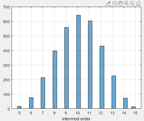
Spurs intermodulation orders histogram:

figure(3);histogram(fint_ord(:,2),2*max(fint_ord(:,2)))

grid on;xlabel('intermod order')

So, IP3 point Input Intermodulation Product 3 or IIP3 is defined by [IIP3 OIP3] and is the input power that would be needed for a given non-linear device to produce same amount of power out of the fundamental coefficient a1, and from the 3rd order coefficient a3 . When Pin=IIP3 then Pout=OIP3

When building a mixer, the interest may be precisely on the amount of power generated on a given harmonic, to then filter out fundamental along with any other harmonic.

abs(a1)<1 is an attenuator.

abs(a1)>1 is an amplifier.

Gv is not power gain but voltage gain.

All coefficients are assumed constant

over frequency because used carriers

are narrowband.

Note that point IP2 can also be defined, out of IIP2 and OIP2 . However as [JASP] shows (next graph right hand side), for an increasing input signal OIP3 is typically reached before OIP2.

Intermodulation orders are proportional to Pin/Pout slope.

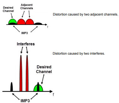
Inter-Modulation Product order 3 or IMP3 , same as Inter-Modulation Distortion order 3 or IMD3 is a common figure of merit obtained through test with one or more adjacent interferers having significantly higher power than the carrier in the desired channel [CAER] , also used to find out how much power analog amplifiers spill out of channel. The result of these measurement, contrasting IP3 measurements, is not the in-out power that equates linear and order 3 power levels, but the power distance between carrier and interferer; the lower the spur the better is the system.

IP3 is also found in literature as Third Order Intercept or TOI .

For f with 2 carriers or interferers, the IP3 relevant intermodulation takes place at abs(2*f(1)-f(2)) and abs(2*f(2)-f(1))

Heading 5

N=3 % linear interm mod order roof for a single carrier

f=[1 2.3]; % [GHz]

size(combinator(N,numel(f),'p','r'),1)* ... size(combinator(2,numel(f),'p','r'),1)

fint=zeros(1,numel(f)+1);

L1=combinator(N,numel(f),'p','r');

for k1=1:1:size(L1,1)

L2=(2*(combinator(2,numel(f),'p','r')-1.5));

L3=L1(k1,:).*f;

O1=sum(abs(L1(k1,:)));

fint=[fint ; L3.*L2 repmat(O1,size(L2,1),1)];

end

fint(1,:)=[];

fint_ord=unique([abs(sum(fint(:,[1:numel(f)]),2)), ...

fint(:,end)],'rows')

For a closer pair of input carriers

f=[2.1 2.3]; % [GHz]

size(combinator(N,numel(f),'p','r'),1)*...

size(combinator(2,numel(f),'p','r'),1)

fint=zeros(1,numel(f)+1);

L1=combinator(N,numel(f),'p','r');

for k1=1:1:size(L1,1)

L2=(2*(combinator(2,numel(f),'p','r')-1.5));

L3=L1(k1,:).*f;

O1=sum(abs(L1(k1,:)));

fint=[fint ; L3.*L2 repmat(O1,size(L2,1),1)];

end

fint(1,:)=[];

fint_ord=unique([abs(sum(fint(:,[1:numel(f)]),2)) fint(:,end)],'rows')

To group spurs according intermodulation order:

sortrows(fint_ord,2)

Another way to build a list with all potential intermodulation products is as follows:

N=3;

f=[1 2.3]*1e9 % [Hz]

n1=[0:1:N];n2=[0:1:N];

F1=repmat(f(1)*n1,N+1,1);

F2=repmat(f(2)*n2,N+1,1)';

T1=abs(F1-F2);

T2=F1+F2;

f0=unique(sort([T1(:)' T2(:)']))

fint_ord =

0.300000000000000 3.000000000000000

0.700000000000000 4.000000000000000

1.300000000000000 2.000000000000000

1.600000000000000 5.000000000000000

2.600000000000000 4.000000000000000

3.300000000000000 2.000000000000000

3.600000000000000 3.000000000000000

3.899999999999999 6.000000000000000

4.300000000000000 3.000000000000000

4.899999999999999 5.000000000000000

5.300000000000000 4.000000000000000

5.600000000000000 3.000000000000000

5.899999999999999 4.000000000000000

6.600000000000000 4.000000000000000

7.600000000000000 5.000000000000000

7.899999999999999 4.000000000000000

8.899999999999999 5.000000000000000

9.899999999999999 6.000000000000000

fint_ord =

0.190000000000000 2.000000000000000

0.380000000000000 4.000000000000000

0.569999999999999 6.000000000000000

1.730000000000000 5.000000000000000

1.920000000000000 3.000000000000000

2.490000000000000 3.000000000000000

...

6.709999999999999 3.000000000000000

8.629999999999999 4.000000000000000

8.820000000000000 4.000000000000000

9.010000000000000 4.000000000000000

10.930000000000000 5.000000000000000

11.119999999999999 5.000000000000000

13.230000000000000 6.000000000000000

T1 =

1.0e+09 *

0 2.1000 4.2000 6.3000

2.3000 0.2000 1.9000 4.0000

4.6000 2.5000 0.4000 1.7000

6.9000 4.8000 2.7000 0.6000

T2 =

1.0e+10 *

0 0.2100 0.4200 0.6300

0.2300 0.4400 0.6500 0.8600

0.4600 0.6700 0.8800 1.0900

0.6900 0.9000 1.1100 1.3200

f0 =

1.0e+09 *

Columns 1 through 6

0 0.3000 0.7000 1.0000 1.3000 1.6000

Columns 7 through 12

2.0000 2.3000 2.6000 3.0000 3.3000 3.6000

Columns 13 through 18

3.9000 4.3000 4.6000 4.9000 5.3000 5.6000

Columns 19 through 24

5.9000 6.6000 6.9000 7.6000 7.9000 8.9000

Column 25

9.9000

.imt tables

T1=F1+F2 is the 1st table supplied in [10] appendix B and T2=abs(F1-F2) is the second table in same reference.

References [10] and [11] focus on intermodulation tables, a.k.a. .imt files for mixer system design.

These files do not contain intermodulation frequencies, assumed known and following the |n(1)*f(1)

±n(2)*f(2) .. ±n(N)*f(N)|

pattern, but only power levels on each intermodulation frequency, presented as in F1+F2 and abs(F1-F2) format.

Note that both M*LOand N*Signal ranges start with [0:1:15] thus already supplying a DC value.

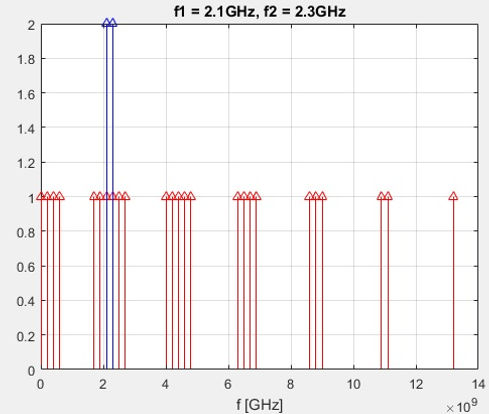
Now let's see how scattered are intermodulation products across spectrum:

Spurs tend to show up around harmonics

figure(4);

h1=stem(f0,ones(1,numel(f0)));

h1.Marker='^';h1.Color='red';

hold on;grid on;

title(['f1 = ' num2str(f(1)/1e9) 'GHz, f2 =' ...

num2str(f(2)/1e9) 'GHz'])

xlabel('f [GHz]')

fflat_in=f/1e9

h2=stem(f,2*ones(1,numel(fflat_in)));

h2.Marker='^';h2.Color='blue'

These 2 graphs only show frequencies, the level is not significant. Input carrier amplitudes all set to 2, all outputs set to 1. The grouping of distortion spurs around harmonics is a bit clearer if the values of f are closer each other.

f=[2.1 2.3]*1e9 % [Hz]

N1=[0:1:N];M1=[0:1:N];

F1=repmat(f(1)*N1,N+1,1)

F2=repmat(f(2)*M1,N+1,1)'

T1=F1+F2

T2=abs(F1-F2)

f0=unique(sort([T1(:)' T2(:)']));

figure(5);

h1=stem(f0,ones(1,numel(f0)));

h1.Marker='^';

h1.Color='red';

hold on;grid on;

title(['f1 = ' num2str(f(1)/1e9) ...

'GHz, f2 = ' num2str(f(2)/1e9) 'GHz'])

xlabel('f [GHz]')

fflat_in=f/1e9

h2=stem(f,2*ones(1,numel(fflat_in)));

h2.Marker='^'

h2.Color='blue'

Sometimes only harmonics, multiples of each frequency, are of interest: n*f(1) n*f(2) .. although occasionally one may read the term 'harmonic' used to point at any of the above linear combinations.

Mind the gap; some literature calls fundamental carriers '1st harmonic(s)' . So does [POZAR] calling 2*f(1) and 2*f(2) respectively 2nd harmonics, implying f(1) and f(2) are 1st harmonics. However one may come across term fundamental for [POZAR] 1st harmonic. Then 1st harmonic actually refers to [POZAR] 2nd harmonic.

Following, let's simulate what IP3 measurements are about when for instance requiring a system to comply with EMC specifications.

SIMULATING IP3 MEASUREMENTS

In RF microwave engineering undergraduate University courses, in the laboratory regarding IP3, one is usually requested to manually obtain a1(Pin,Pout) and a3(Pin,Pout) by gradually increasing input power, building in-out power graphs for F1 (or F2) and for 2*F1-F2 (or 2*F2-F1).

For amplifiers when Pin/Pout slope starts decreasing then it's time to look for IP1dB 1dB compression point,

IP1dB=[IIP1dB OIP1dB].

Generating Signals

T=min(1./f)

dt=T/100 % time resolution, way above Nyquist limit to avoid low resolution

t=[0:dt:20*T]; % amount of cycles to simulate, 20 cycles of slowest frequency

Fs=1/dt

Voltage or current signals, measuring their power and discerning power for each intermodulation component with spectrum analysis, these are all needed measurements to know IP3. Assuming Non-linear narrow band coefficients a1 a2 .. then these coefficients are usually considered constant over frequency. A 1st approach could be single carrier input:

a0=1;a1=3;a2=.8;a3=.6;

V0=1 % pg513

vi=V0*sum(cos(2*pi*f'.*t)) % input 2 carriers

vo1=a1*vi;

vo2=a0+a1*vi+a2*vi.^2+a3*vi.^3; % output

figure(6)

plot(t,vi);

hold on

plot(t,vo1);ax6=gca

xlabel('t [s]');

legend({'v_i(t)','v_o(t)'})

grid on;

title('Linear System v_o=G_v*v_i=a_1*v_i')

The previous system is the linear part of completely linear of vo2=a0+a1*vi+a2*vi.^2+a3*vi.^3 . Linear systems preserve zero crossings through, input and output signals are completely proportional.

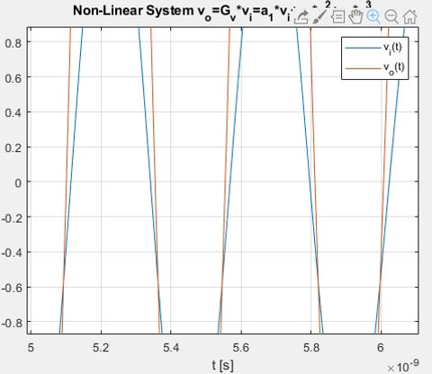
Now, Input group of carriers to non-linear system, all same amplitude but different frequencies:

figure(7)

plot(t,vi);

hold on

plot(t,vo2);ax7=gca

xlabel('t [s]');

legend({'v_i(t)','v_o(t)'})

grid on;

title('Non Linear System ,,,

v_o=G_v*v_i=a_1*v_i+a_2*v_i^2+a_3*v_i^3')

ax6.DataAspectRatio=ax7.DataAspectRatio

linear part of another example, now null DC and all AC components same amplitude:

a0=0;a1=-2;a2=.2;a3=2;

V0=1

vi=V0*sum(cos(2*pi*f'.*t)) % input 2 carriers

vo1=a1*vi;

vo2=a0+a1*vi+a2*vi.^2+a3*vi.^3; % output

figure(8)

plot(t,vi);

hold on

plot(t,vo1);ax8=gca

xlabel('t [s]');

legend({'v_i(t)','v_o(t)'})

grid on;

title('Linear System vo=Gv*vi=a1*vi')

figure(9)

plot(t,vi);

hold on

plot(t,vo2);ax9=gca

xlabel('t [s]');

legend({'v_i(t)','v_o(t)'})

grid on;

title('Non Linear System ...

v_o=G_v*v_i=a_1*v_i+a_2*v_i^2+a_3*v_i^3')

ax8.DataAspectRatio=ax9.DataAspectRatio

Test Instrument simulator dsp.SpectrumAnalyzer

So, the system model has to do with voltage or current signals through a narrow band non-linear model, but IP3=[IIP3 OIP3] are power measurements, and often the actual IIP3 OIP3 values are not even calculated or measured, leaving it to measuring peaks distance between carrier and |2*f1-f2| or |2*f2-f1|, to reach compliance for instance towards certification, for a product to be sold in a market.

Often IP3 reports skip the last part, supplying dBc measurement between peaks as the actual IP3, leaving the actual calculation as obvious.

RF Power measurements mean averaging.

There is a concept of instantaneous power p(t) = v(t)*i(t) but if mentioned in literature, it's usually a mere footnote. Because for cyclic signals, to measure average power it only makes sense to average at least over one period, and actually if possible over a 'large' amount of signal periods.

Since we are using diverse frequencies, there are multiple signal periods to be taken into account, one for each carrier, but just going for twice the shortest one is not good enough to achieve correct measurements.

Use to automatically place SA markers on peaks.

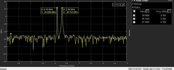
A 1/2V amplitude sine carrier (on Z0=1W) has 1/8W RF power = -9dBW = 21dBm(W) .

With dsp.SpectrumAnalyzer of a pair of 1/2V amplitude carriers is:

Fs2=Fs/20

Nspf=4*1024

Sineobject1 = ...

dsp.SineWave('SamplesPerFrame',Nspf, ...

'SampleRate',Fs2, ...

'Frequency',f(1), ...

'Amplitude',.5);

Sineobject2 = ...

dsp.SineWave('SamplesPerFrame',Nspf, ...

'SampleRate',Fs2, ...

'Frequency',f(2), ...

'Amplitude',.5);

SA = dsp.SpectrumAnalyzer('SampleRate',Fs2, ...

'Name','fig.10 : Spectrum Analyser 01', ...

'Method','Filter bank',...

'SpectrumType','Power',...

'PlotAsTwoSidedSpectrum',true,...

'ChannelNames',{'S_i(f)'}, ...

'YLimits',[-120 40], ...

'ShowLegend',true);

data = [];

for Iter = 1:3000

Sinewave1 = Sineobject1();

Sinewave2 = Sineobject2();

Input = Sinewave1 + Sinewave2;

NoisyInput = Input + 0.001*randn(Nspf,1);

SA(NoisyInput);

if SA.isNewDataReady

data = [data;getSpectrumData(SA)];

end

release(SA);

Same signal over one sided spectrum is going to show double power levels than when on 2-sided spectrum.

Let's do it: folding spectrum, one sided display doubles (+3dB) power reading because now all signal power only spreads over one side of the display.

SA = dsp.SpectrumAnalyzer('SampleRate',Fs2, ...

'Method','Filter bank', ...

'SpectrumType','Power', ...

'PlotAsTwoSidedSpectrum',false, ...

'ChannelNames',{'S_i(f)'}, ...

'YLimits',[-120 40], ...

'ShowLegend',true);

SA.FrequencySpan='Start and stop frequencies'

SA.StartFrequency=2e5

SA.StopFrequency=5e9

data = [];

for Iter = 1:3000

Sinewave1 = Sineobject1();

Sinewave2 = Sineobject2();

Input = Sinewave1 + Sinewave2;

NoisyInput = Input + 0.001*randn(Nspf,1);

SA(NoisyInput);

if SA.isNewDataReady

data = [data;getSpectrumData(SA)];

end

release(SA);

dsp.SpectrumAnalyzer key parameters

Sampling Rate I set it to a number near Fs to avoid not supplying enough input data to SA

SA.SampleRate

Fs

Fs2

=

1.150000000000000e+10Fs =

Fs =

2.300000000000000e+11

Fs2 =

1.150000000000000e+10

Resolution Bandwidth, like on any real Spectrum Analyser. Change SA.RBWSource='Property' for FFT parameters to control of frequency resolution. SA.RBW default value is 9.76 .

SA.RBW

=

20000000

Frequency Span may be defined in one of the following ways: full | [start stop] or [centre span]

SA.Span

=

5.750000000000000e+09

To avoid losing frequency resolution the following has to be true

SA.Span/SA.RBW>2

With SA.RBWSource='Auto' this key parameter RBW is always controlled by SA

Even when attempting SA.FrequencyResolutionMethod='RBW'

if SA.RBWSource='Auto' then SA ignores any number manually assigned to RBW.

Sometimes for heavy computing load or/and limited CPU a calculated reduction of frequency resolution may be reasonable. However, RBW defines frequency resolution, so if too coarse the measurement may not render meaningful or even misleading results.

Here for instance, apply the following: SA.RBWSource='Property'; SA.RBW=2e8; run again the last code block on page 9, and zoom on any of the carrier peaks.

For my platform SA.RBW=20 this is RBW=20 %Hz is too demanding for the amount of time to wait for the SA to start displaying calculated traces.

But for RBW=2 %kHz I get this:

Note that despite Sample rate SA.SampleRate set to Fs2 now SA has pushed it up beyond 11GHz to meet frequency resolution below assigned RBW=20 %Hz.

So now the frequency accuracy is impeccable, look at the really sharp peaks.

A single frequency sample right on each f value, yet the power accuracy now has gone to the wall: -75dBm !? the input signal is composed of 2 carriers, each with 0.125W.

=

logical

1

DSPs FPGAs ... have pushed to a corner analog signal processing; what in the 70s had to be done with hardware, by the 90s could be implemented with software. So instead of actually sweeping a narrow filter that defines frequency resolution, one can apply for instance FFT and obtain similarly accurate spectrum measurement results.

FrequencyResolutionMethod has 3 states: [RBW WindowLength NumFrequencyBands]

SA.NumFrequencyBands : only considered when SA.Method='Filter bank'

then use SA.FFTLengthSource ['Auto' | 'Property'] and SA.FFTLength (1024 default) to

control frequency resolution.

SA.WindowLength : only considered when SA.Method='Welch'

then use SA.WindowLength to control frequency resolution through amount of FFT points.

Example with SA.Method='Welch' , Welch RBW window is an improvement to the Barlett RBW window in regards that overlapping is allowed, improving accuracy, that may be then lost if the overlap queue is too long, observe wider carrier precisely because of the overlap.

SA = dsp.SpectrumAnalyzer

SA.Name='fig.12 : Spectrum Analyser 01'

SA.SampleRate=Fs2

SA.Method='Welch' % changed RBW window

SA.SpectrumType='Power'

SA.PlotAsTwoSidedSpectrum=false

SA.ChannelNames={'S_i(f)'}

SA.YLimits=[-120 40]

SA.ShowLegend=true

SA.FrequencySpan='Start and stop frequencies'

SA.StartFrequency=2e5

SA.StopFrequency=5e9

SA.FrequencyResolutionMethod='WindowLength'

SA.FFTLengthSource='Property'

SA.FFTLength=1024

data = [];

for Iter = 1:3000

Sinewave1 = Sineobject1();

Sinewave2 = Sineobject2();

Input = Sinewave1 + Sinewave2;

NoisyInput = Input + 0.001*randn(Nspf,1);

SA(NoisyInput);

if SA.isNewDataReady

data = [data;getSpectrumData(SA)];

end

SA = dsp.SpectrumAnalyzer

SA.Name='fig.13 : Spectrum Analyser 01'

SA.SampleRate=Fs2

SA.Method='Welch'

SA.SpectrumType='Power'

SA.PlotAsTwoSidedSpectrum=false

SA.ChannelNames={'S_i(f)'}

SA.YLimits=[-120 40]

SA.ShowLegend=true

SA.FrequencySpan='Start and stop frequencies'

SA.StartFrequency=2e5

SA.StopFrequency=5e9

SA.FrequencyResolutionMethod='WindowLength'

SA.FFTLengthSource='Property'

SA.FFTLength=8*1024 % increased FFTLength

data = [];

for Iter = 1:3000

Sinewave1 = Sineobject1();

Sinewave2 = Sineobject2();

Input = Sinewave1 + Sinewave2;

NoisyInput = Input + 0.001*randn(Nspf,1);

SA(NoisyInput);

if SA.isNewDataReady

data = [data;getSpectrumData(SA)];

end

how to close dsp.SpectrumAnalyzer objects

release(SA) % this just releases RAM but SA still in workspace

delete(SA) % there's no close(SA), use delete(SA)

Apply 1/50 to power readings in order to take into account common Z0=50 or -10*log10(50)=-16.9897 on either dBm(W) or dB(W) .

Spectrum Analyser measurement simulation examples with simulink

Mathworks has simulink example [4] that simulates important RF interference parameters:

SpectrumAnalyzerMeasurementsExample

While

Adjacent Channel Power Ratio (ACPR)
Complementary Cumulative Distribution Function (CCDF)

are popular and useful RF channel measurements, regarding example 10.4 the important ones are:

Intermodulation Distortion
Harmonic Distortion

Harmonic Distortion

Intermodulation Distortion

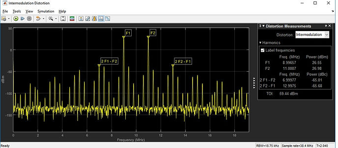
Let's focus on 3rd order intermodulation.

SpectrumAnalyzerMeasurementsExample3

I have changed the amplifier model Amplifier2

coefficients to a0=0;a2=0 and a1=1;a3=1

In both sine wave generator blocks change

Amplitude to required value in order to obtain

a simulated output distortion.

With this particular Simulink example, I have changed span mode to FStart 1GHz and FStop 8GHz. Both input signals are oversampled at considerably higher rate than f=1e9*[2.1 2.3] . Under-sampling noise modelled inside Amplifier2 effectively removes it at the input showing purely intermodulation only.

When adding noise (change noise sampling to for instance to 1/10/3/86e10 similar sampling value on input signals) one realises how important is for a system to be as quiet as possible to avoid apparently low level intermodulation products not to be lifted as shown now on right hand side:

TOI is quite the same, without noise 43.49dBm, with noise 44.36dBm, but with noise there's a bunch of spurs populating band around

f=1e9*[2.1 2.3]

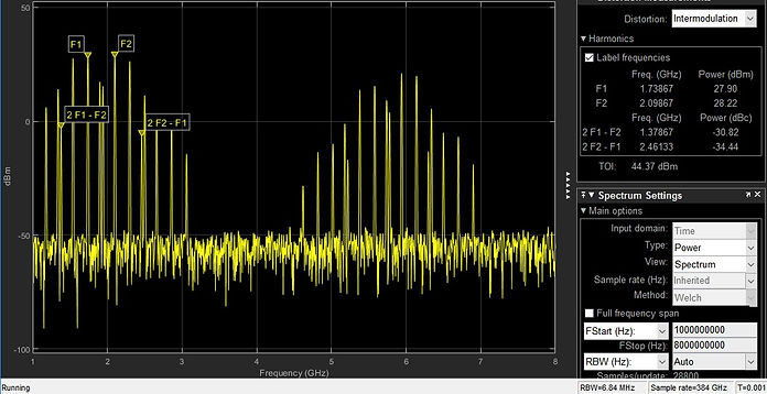
On gradually increasing input power, one realises that the [dBc] measurement difference between adjacent peaks goes from about -15dB difference between power levels F1 and F2 against power levels of 2*F1 - F2 and 2*F2 - F1, up to something like -9dBc.

But then, on further increasing input power, no matter how much power, whatever insane amount of Watts one puts in, even setting the amplifier coefficients to [1 0 .01 0] this is a3=1;a2=0; a1=.01;a0=0 there's no way to bring such peaks difference any closer.

So by playing these simple simulink examples one can appreciate the eventual compression that takes place when arbitrarily increasing input power, such compression preventing from bringing output 2*F1 - F2 and/or 2*F2 - F1 peaks up to same level of F1 F2 peaks: All systems have limits.

Spectrum peaks capture - constant input level

One could certainly process time traces with findpeaks but dsp.SpectrumAnalyzer includes peaks capture with corresponding frequencies.

After a bit of reading I learnt how directly capture peak measurements with the following

%% SYSTEM

a_coeff=[.12 -.4 12 .5]

%% TIME FRAME

f=[2.1 2.3]*1e9 % [Hz] input carriers

Fs = 10*f(2); % sampling rate

Nspf=4096 % samples per frame

%% INPUT CARRIERS

Sineobject1 = dsp.SineWave

Sineobject1.SamplesPerFrame=2*1024

Sineobject1.PhaseOffset=0

Sineobject1.SampleRate=Fs

Sineobject1.Frequency=f(1) % /1e3, test no need trick to work with kHz to reduce amount operations

Sineobject1.Amplitude=.5 % 1/2 amplitude [V]

Sineobject2 = dsp.SineWave

Sineobject2.SamplesPerFrame=2*1024

Sineobject2.PhaseOffset=0

Sineobject2.SampleRate=Fs

Sineobject2.Frequency=f(2) % /1e3 no need

Sineobject2.Amplitude=.5 % 1/2 amplitude [V]

%% TEST INSTRUMENT

SA2 = dsp.SpectrumAnalyzer

SA2.Name='fig.14 : Spectrum Analyser 02'

SA2.SampleRate=Fs

SA2.Method='Filter bank'

SA2.SpectrumType='Power'

SA2.PlotAsTwoSidedSpectrum=false

SA2.ChannelNames={'S_in(f)'}

SA2.YLimits=[-120 90]

SA2.ShowLegend=true

SA2.CursorMeasurements.Enable = true;

SA2.ChannelMeasurements.Enable = true;

SA2.PeakFinder.Enable = true;

SA2.PeakFinder.NumPeaks=14

SA2.PeakFinder.MinDistance=8 % distance in number of samples SA3.PeakFinder.Threshold= % min height difference of peak with

% neighbouring peaks, don't set in case neighbouring peaks have similar levels.

SA2.PeakFinder.MinHeight= -40 % [dBm] squelch, do not detect below this level

SA2.DistortionMeasurements.Enable = true;

%% DAQ LOOP 1

data_measurement = [];

for Iter = 1:1000

st1 = Sineobject1();

st2 = Sineobject2();

s_in2 = a_coeff(1)*ones(numel(st1),1)+...

a_coeff(2)*(st1 + st2)+...

a_coeff(3)*(st1.*st1+st2.*st2+2*st1.*st2)+...

a_coeff(4)*(st1.*st1.*st1+st2.*st2.*st2+...

3*st1.*st1.*st2+3*st2.*st2.*st1)+...

0.001*randn(numel(st1),1);

SA2(s_in2);

if SA2.isNewDataReady

data_measurement = [data_measurement;getMeasurementsData(SA2)];

end

release(SA2)

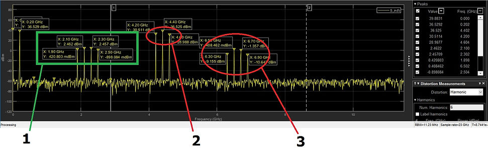
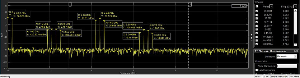
Reached this point and after all above said, it's reasonable to focus on the frequencies around f=[2.1 2.3]*1e9 % Hz

At one point or another any RF system involving a similar system to the one modeled with a_coeff is going to need filters to reject 2 and 3.

data_measurement is a table with the following format

data_measurement

SimulationTime PeakFinder CursorMeasurements ChannelMeasurements DistortionMeasurements

______________ ____________ __________________ ___________________ ______________________

[ 0] [1x1 struct] [1x1 struct] [1x1 struct] [1x1 struct]

[8.904347826086956e-08] [1x1 struct] [1x1 struct] [1x1 struct] [1x1 struct]

[1.780869565217391e-07] [1x1 struct] [1x1 struct] [1x1 struct] [1x1 struct]

..

Sample, reading trace out of last (highest) input ramp level

%% DATA PROCESSING 1

peakvalues = data_measurement.PeakFinder(end).Value

peakvalues =

39.883087676450756

36.528991730620540

36.524982090685270

30.511291762260498

28.988041890041544

2.469926213599443

2.451947690862092

0.405921905564615

0.390764568633330

-0.911952645080348

-1.341820682695701

-9.138656004038396

-10.673216421877015

f_peaks_Hz = data_measurement.PeakFinder(end).Frequency

f_peaks_Hz = 1.0e+09 *

0

0.202148437500000

4.402343750000000

4.200195312500000

4.604492187500000

2.100097656250000

2.302246093750000

1.897949218750000

6.502441406250000

2.504394531250000

6.704589843750000

6.300292968750000

6.895507812500000

Tried to put next to data_measurement = [data_measurement; getMeasurementsData(SA2)]; a 2nd log update append for traces data_f_trace = [data_f_trace; getSpectrumData(SA2)] but it seems that another DAQ loop is needed to collect the 2nd log.

%% DAQ LOOP 2

% data_measurement = [];

data_f_trace = [];

for Iter = 1:1000

st1 = Sineobject1();

st2 = Sineobject2();

s_in2 = a_coeff(1)*ones(numel(st1),1)+...

a_coeff(2)*(st1 + st2)+...

a_coeff(3)*(st1.*st1+st2.*st2+2*st1.*st2)+...

a_coeff(4)*(st1.*st1.*st1+st2.*st2.*st2+...

3*st1.*st1.*st2+3*st2.*st2.*st1)+...

0.001*randn(numel(st1),1);

SA2(s_in2);

if SA2.isNewDataReady

data_f_trace = [data_f_trace; getSpectrumData(SA2)]

end

So DAQ loop 1 collects SA measurements data, and DAQ loop 2 collects the actual power spectrum traces.

%% DATA PROCESSING 2

data_f_trace.Spectrum % [dBm] traces

=

21×1 cell array

{1025×1 double}

..

F=data_f_trace.FrequencyVector{1}'

S=zeros(size(data_f_trace.Spectrum,1), ...

size(data_f_trace.Spectrum{1},1));

for k=1:1:size(data_f_trace.Spectrum,1)

S(k,:)=data_f_trace.Spectrum{k}';

end

% S1 is just a sample

S1=mean(S);

figure;plot(F,S1);grid on

xlabel('f');ylabel('output [dBmW]')

[pks,locs]=findpeaks(S1,'MinPeakProminence',40)

hold on

plot(F(locs),pks,'or');grid on;axis tight

F(locs)

pks

F =

1.0e+10 *

Columns 1 through 3

0 0.001123046875000 0.002246093750000

Columns 4 through 6

0.003369140625000 0.004492187500000 0.005615234375000

Columns 7 through 9

0.006738281250000 0.007861328125000 0.008984375000000

Columns 10 through 12

..

Columns 1018 through 1020

1.142138671875000 1.143261718750000 1.144384765625000

Columns 1021 through 1023

1.145507812500000 1.146630859375000 1.147753906250000

Columns 1024 through 1025

1.148876953125000 1.150000000000000

F(locs)

=

1.0e+09 *

Columns 1 through 3

0.202148437500000 1.897949218750000 2.100097656250000

Columns 4 through 6

2.302246093750000 2.504394531250000 4.200195312500000

Columns 7 through 9

4.402343750000000 4.604492187500000 6.300292968750000

Columns 10 through 12

6.502441406250000 6.704589843750000 6.895507812500000

pks =

Columns 1 through 3

36.529249580846511 0.414153814305308 2.468719792275216

Columns 4 through 6

2.451227799072633 -0.916097175031396 30.511429558603652

Columns 7 through 9

36.524942116869475 28.987804890601446 -9.148288828975225

Columns 10 through 12

0.405732788361604 -1.356090060053109 -10.668713020371428

In this example, with gradually increasing input power, findpeaks filter MinPeakProminence is tricky because with constant input I visually chose it to be 40 but once input power level seep is in place, for shorter peaks such threshold has to be smaller otherwise findpeaks misses values needed to be taken into account.

Spectrum peaks capture - input ramp

%% SYSTEM

a_coeff=[.12 -.4 12 .5]

Z0=1

%% TIME FRAME

f=[2.1 2.3]*1e9 % [Hz] input carriers

Fs = 10*f(2); % sampling rate

Nspf=4096 % samples per frame

%% INPUT CARRIERS

Sineobject1 = dsp.SineWave

Sineobject1.SamplesPerFrame=2*1024

Sineobject1.PhaseOffset=0

Sineobject1.SampleRate=Fs

Sineobject1.Frequency=f(1)

Sineobject2 = dsp.SineWave

Sineobject2.SamplesPerFrame=2*1024

Sineobject2.PhaseOffset=0

Sineobject2.SampleRate=Fs

Sineobject2.Frequency=f(2)

%% TEST INSTRUMENT

SA3 = dsp.SpectrumAnalyzer

SA3.Name='fig.16 : Spectrum Analyser 03'

SA3.SampleRate=Fs

SA3.Method='Filter bank'

SA3.SpectrumType='Power'

SA3.PlotAsTwoSidedSpectrum=false

SA3.ChannelNames={'S_in(f)'}

SA3.YLimits=[-80 110]

SA3.ShowLegend=true

SA3.CursorMeasurements.Enable = true;

SA3.ChannelMeasurements.Enable = true;

SA3.PeakFinder.Enable = true;

SA3.PeakFinder.NumPeaks=14

SA3.PeakFinder.MinDistance=8 % distance in number of samples SA4.PeakFinder.Threshold= % min height difference of peak with

% neighbouring peaks, don't set in case neighbouring peaks have similar levels.

SA3.PeakFinder.MinHeight= -40 % [dBm] squelch, do not detect below this level

SA3.DistortionMeasurements.Enable = true;

N_iter=1e3 % amount of time to repeat sweep with same input power

%% RAMP

N0_dBm=-60 % visual inspection, noise floor fairly flat at -60dBmW/Hz

% change start stop input power values to adjust test window

Pin_start=10^((N0_dBm-30)/10) % [W] start ramp

Pin_stop=1e2 % [W] stop ramp

Pin_start_dBm=10*log10(Pin_start)+30 % [dBmW] start ramp

Pin_stop_dBm=10*log10(Pin_stop)+30 % stop ramp

N_ramp=30 % choose amount of levels, ramp resolution

ramp1_dBm=linspace(Pin_start_dBm,Pin_stop_dBm,N_ramp) % input power ramp [dBmW]

ramp1_W=10.^((ramp1_dBm-30)/10) % input power ramp [W]

ramp1_V_Z0=(ramp1_W*2*Z0).^.5

%% DAQ LOOP 3

data_measurement = [];

% data_f_trace = [];

for k=1:1:numel(ramp1_V_Z0)

Sineobject1.Amplitude=ramp1_V_Z0(k)

Sineobject2.Amplitude=ramp1_V_Z0(k)

for Iter = 1:N_iter

st1 = Sineobject1();

st2 = Sineobject2();

s_in2 = a_coeff(1)*ones(numel(st1),1)+...

a_coeff(2)*(st1 + st2)+...

a_coeff(3)*(st1.*st1+st2.*st2+2*st1.*st2)+...

a_coeff(4)*(st1.*st1.*st1+st2.*st2.*st2+...

3*st1.*st1.*st2+3*st2.*st2.*st1)+...

0.001*randn(numel(st1),1);

SA3(s_in2);

if SA3.isNewDataReady

data_measurement = [data_measurement;getMeasurementsData(SA3)];

% data_f_trace = [data_f_trace;getSpectrumData(SA4)];

end

No need to elaborate on the fact that not many RF systems can accurately generate carriers from -60dBm(W) up to 96dBm(W) = 4MW RF power.

There are critical factors not considered in chapter 10 to take into account like cooling, load capacity to stand delivered power, for how long has the load to stand peak power .. and the critical module that supports them all: power supply;

No RF system can deliver more power than a fraction of the power made available by its power supply. Safety measures have to be implemented to avoid power supply overload.

First I am sampling to understand data format:

%% DATA PROCESSING 3

[sz1 sz2]=size(data_measurement.PeakFinder)

% samples

peakvalues = data_measurement.PeakFinder(1).Value'

f_peaks_Hz = data_measurement.PeakFinder(1).Frequency'

peakvalues = data_measurement.PeakFinder(floor(sz1/4)).Value'

f_peaks_Hz = data_measurement.PeakFinder(floor(sz1/4)).Frequency'

peakvalues = data_measurement.PeakFinder(floor(sz1/2)).Value'

f_peaks_Hz = data_measurement.PeakFinder(floor(sz1/2)).Frequency'

peakvalues = data_measurement.PeakFinder(floor(3*sz1/4)).Value'

f_peaks_Hz = data_measurement.PeakFinder(floor(3*sz1/4)).Frequency'

peakvalues = data_measurement.PeakFinder(end).Value'

f_peaks_Hz = data_measurement.PeakFinder(end).Frequency'

Since I reduced N_iter to in turn reduce simulation time, just to solve in time for this particular example, just and example having reached 30 pages, floor(n*sz1) is also useful to then index at chosen fraction of the amount of traces generated.

When input signal low enough no peaks, or just input f carriers are spotted.

As soon as input carriers power above certain level, F1 F2 2F1-F2 and 2F2-F1 clearly show on either display and are caught by the Spectrum Analyser as peak measurements.

But then, with input power further increasing, additional peaks are included in the measurement that are neither needed nor relevant to TOI measurements

sz1 =

66

sz2 =

1

peakvalues =

1×0 empty double row vector

f_peaks_Hz =

1×0 empty double row vector

peakvalues =

Columns 1 through 3

11.730668054087094 -18.622243685427840 -18.668098767746685

Columns 4 through 6

-26.808670662280221 -26.811246826302295 -32.468723034362725

Column 7

-34.833043456620615

f_peaks_Hz =

1.0e+09 *

Columns 1 through 3

0 2.302246093750000 2.100097656250000

Columns 4 through 6

0.202148437500000 4.402343750000000 4.200195312500000

Column 7

4.604492187500000

peakvalues =

Columns 1 through 3

30.697825644004304 26.354370234072729 26.291946629849996

Columns 4 through 6

20.644444302502801 18.201466879088851 5.935358751747067

Columns 7 through 9

5.772574498859978 -14.837519555557776 -14.970952554129902

Columns 10 through 12

-16.918553125171840 -17.409025860269267 -24.082041973679367

Column 13

-26.652811335452682

f_peaks_Hz =

1.0e+09 *

Columns 1 through 3

0 0.202148437500000 4.402343750000000

Columns 4 through 6

4.200195312500000 4.604492187500000 2.100097656250000

Columns 7 through 9

2.302246093750000 1.897949218750000 6.502441406250000

Columns 10 through 12

2.504394531250000 6.704589843750000 6.300292968750000

Column 13

6.895507812500000

peakvalues =

Columns 1 through 3

44.596909142718047 41.591079391306081 41.586563952348072

Columns 4 through 6

35.372716404153628 33.807563160241351 7.977940042372850

Columns 7 through 9

7.956704562909529 6.375958161169194 5.905691878305284

Columns 10 through 12

3.648219321271647 2.858947600331962 -1.803748308661298

Column 13

-3.392408218381100

f_peaks_Hz =

1.0e+09 *

Columns 1 through 3

0 4.402343750000000 0.202148437500000

Columns 4 through 6

4.200195312500000 4.604492187500000 6.502441406250000

Columns 7 through 9

1.897949218750000 2.504394531250000 6.704589843750000

Columns 10 through 12

2.302246093750000 2.100097656250000 6.300292968750000

Column 13

6.895507812500000

peakvalues =

Columns 1 through 3

90.016693316545954 87.003553778432661 86.998579041436116

Columns 4 through 6

85.624389041214869 85.620546229610440 80.985013535730644

Columns 7 through 9

79.463526674474465 76.119255118760492 76.108505146928536

Columns 10 through 12

74.809066602405835 74.363724178781496 66.577247608746063

Column 13

65.055932136076819

f_peaks_Hz =

1.0e+09 *

Columns 1 through 3

0 0.202148437500000 4.402343750000000

Columns 4 through 6

2.100097656250000 2.302246093750000 4.200195312500000

Columns 7 through 9

4.604492187500000 1.897949218750000 6.502441406250000

Columns 10 through 12

2.504394531250000 6.704589843750000 6.300292968750000

Column 13

6.895507812500000

Let's work directly on spectrum traces:

%% DAQ LOOP 4

% data_measurement = [];

data_f_trace = [];

for k=1:1:numel(ramp1_V_Z0)

Sineobject1.Amplitude=ramp1_V_Z0(k)

Sineobject2.Amplitude=ramp1_V_Z0(k)

for Iter = 1:N_iter

st1 = Sineobject1();

st2 = Sineobject2();

s_in2 = a_coeff(1)*ones(numel(st1),1)+...

a_coeff(2)*(st1 + st2)+...

a_coeff(3)*(st1.*st1+st2.*st2+2*st1.*st2)+...

a_coeff(4)*(st1.*st1.*st1+st2.*st2.*st2+...

3*st1.*st1.*st2+3*st2.*st2.*st1)+...

0.001*randn(numel(st1),1);

SA4(s_in2);

if SA4.isNewDataReady

% data_measurement = [data_measurement;getMeasurementsData(SA4)];

data_f_trace = [data_f_trace;getSpectrumData(SA4)];

end

Now we have captured all measurement peaks and their respective frequency positions directly from dsp.Spectrum.Analyzer .

However, obtained peak amount per trace is not the same for all traces.

Next, removing odd traces:

%% DATA PROCESSING 4

data_f_trace

F=data_f_trace.FrequencyVector{1};

data_f_trace.Spectrum; % [dBm]

data_f_trace.FrequencyVector; % [Hz]

size(data_f_trace,1)

data_f_trace =

866×3 table

SimulationTime Spectrum FrequencyVector

___________________ _______________ _______________

[0.002671304347826] [1025×1 double] [1025×1 double]

[0.002671393391304] [1025×1 double] [1025×1 double]

...

= 183 3

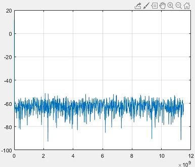
figure(17);

plot(F,data_f_trace.Spectrum{1)});

grid on;xlabel('f');title('output sample 1/3rd ramp')

figure(17);

plot(F,data_f_trace.Spectrum{2)});

grid on;xlabel('f');title('output sample 1/3rd ramp')

figure(17);

plot(F,data_f_trace.Spectrum{floor(size(data_f_trace,1)/20)});

grid on;xlabel('f');title('output sample 1/3rd ramp')

hf18=figure(18);

plot(F,data_f_trace.Spectrum{floor(2*size(data_f_trace,1)/3)});

ax18=gca; grid on;xlabel('f');title('output sample 2/3rd ramp')

S=zeros(size(data_f_trace.Spectrum,1),size(data_f_trace.Spectrum{1},1));

for k=1:1:size(data_f_trace.Spectrum,1)

S(k,:)=data_f_trace.Spectrum{k}';

end

size(S)

figure(19);

for k=1:1:size(S,1)

plot(F,S(k,:));

hold on;

end

xlabel('f');ylabel('output [dBmW]');grid on

%% odd traces out

S([1:2],:)=[]

close(hf19)

figure(19);

for k=1:1:size(S,1)

plot(F,S(k,:));

hold on;

end

xlabel('f');ylabel('output [dBmW]');grid on

size(ramp1_W,2)

% but

size(S,1)

S1=data_f_trace.Spectrum{floor(2*size(data_f_trace,1)/3)};

[pks,locs]=findpeaks(S1,'MinPeakProminence',15)

hold(ax18,'on')

plot(ax18,F(locs),pks,'or');grid on;axis tight

F(locs);

pks;

[pks,locs]=findpeaks(S1,'MinPeakProminence',25)

hold(ax18,'on')

plot(ax18,F(locs),pks,'dg','MarkerSize',10);grid on;axis tight

F(locs);

pks;

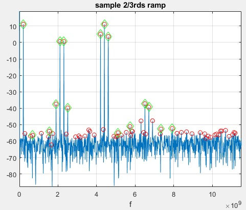
S contains all useful traces. However, as findpeaks used here, too many false peaks.

findpeaks with MinPeakProminence requires a changing threshold, along with ramp otherwise false peaks are taken into account.

Let's have a look at the input ramp. It would be useful to get somehow an amount of measurements proportional to amount ramp levels to then draw in-out power curves. But because the ramp starts below noise ground, there are void measurements.

figure;stem(ramp1_W);grid on

title('input ramp [W]')

figure;stem(10*log10(ramp1_W)+30);grid on

title('input ramp [dBm(W)]')

Let's pull up input ramp 1st level from -60dBm up to -20dBm. Compressing the input ramp; same amount of steps, same stop input power, but higher ramp start input power.

%% RAMP 2

N01=-20; % [dBmW]

Pin_start2=10^((N01-30)/10); % [W] start ramp

Pin_stop2=1e2; % [W] stop ramp

Pin_start2_dBm=10*log10(Pin_start2)+30; % [dBmW] start ramp

Pin_stop2_dBm=10*log10(Pin_stop2)+30; % stop ramp

N_ramp=30; ramp2_dBm=linspace(Pin_start2_dBm,Pin_stop2_dBm,N_ramp);

ramp2_W=10.^((ramp2_dBm-30)/10);

ramp2_V_Z0=(ramp2_W*2*Z0).^.5;

hold(ax21,'on');stem(ax21,10*log10(ramp2_W)+30,'r')

Narrowing band to [1 3] GHz this way only 2F1-F2, 2F2-F1, F2, F1 show up:

%% DAQ LOOP 5

SA3.FrequencySpan='Start and stop frequencies'

SA3.StartFrequency=1e9

SA3.StopFrequency=3e9

SA3.PeakFinder.NumPeaks=4

disp('getting measurements')

data_measurement3 = [];

for k=1:1:numel(ramp2_V_Z0)

Sineobject1.Amplitude=ramp2_V_Z0(k)

Sineobject2.Amplitude=ramp2_V_Z0(k)

for Iter = 1:N_iter

st1 = Sineobject1();

st2 = Sineobject2();

s_in2 = a_coeff(1)*ones(numel(st1),1)+...

a_coeff(2)*(st1 + st2)+...

a_coeff(3)*(st1.*st1+st2.*st2+2*st1.*st2)+...

a_coeff(4)*(st1.*st1.*st1+st2.*st2.*st2+...

3*st1.*st1.*st2+3*st2.*st2.*st1)+...

0.001*randn(numel(st1),1);

SA3(s_in2);

if SA3.isNewDataReady

data_measurement3 = ...

[data_measurement3;getMeasurementsData(SA3)];

end

DAQ loop 6 is to, instead of raking every single trace that SA supplies, try average output trace from same input ramp level.

%% DAQ LOOP 6

SA4 = dsp.SpectrumAnalyzer

SA4.Name='fig.22 : Spectrum Analyser 04'

SA4.SampleRate=Fs

SA4.Method='Filter bank'

SA4.SpectrumType='Power'

SA4.PlotAsTwoSidedSpectrum=false

SA4.ChannelNames={'S_in(f)'}

SA4.YLimits=[-80 110]

SA4.ShowLegend=true

SA4.CursorMeasurements.Enable = true;

SA4.ChannelMeasurements.Enable = true;

SA4.PeakFinder.Enable = true;

SA4.PeakFinder.NumPeaks=14

SA4.PeakFinder.MinDistance=8

SA4.PeakFinder.MinHeight= -40

SA4.DistortionMeasurements.Enable = true;

SA4.FrequencySpan='Start and stop frequencies'

SA4.StartFrequency=1e9

SA4.StopFrequency=3e9

SA4.PeakFinder.NumPeaks=4

D3v=zeros(1,SA4.FFTLength+1); % log trace values

D3f=zeros(1,SA4.FFTLength+1); % log trace frequencies

for k=1:1:numel(ramp2_V_Z0)

data_f_trace3 = [];

Sineobject1.Amplitude=ramp2_V_Z0(k)

Sineobject2.Amplitude=ramp2_V_Z0(k)

for Iter = 1:1e3

st1 = Sineobject1();

st2 = Sineobject2();

s_in2 = a_coeff(1)*ones(numel(st1),1)+...

a_coeff(2)*(st1 + st2)+...

a_coeff(3)*(st1.*st1+st2.*st2+2*st1.*st2)+...

a_coeff(4)*(st1.*st1.*st1+st2.*st2.*st2+...

3*st1.*st1.*st2+3*st2.*st2.*st1)+...

0.001*randn(numel(st1),1);

SA4(s_in2);

if SA4.isNewDataReady

data_f_trace3 = [data_f_trace3;getSpectrumData(SA4)];

end

szt1=size(data_f_trace3.Spectrum{1},1)

numel(data_f_trace3.Spectrum{1})

L21=zeros(1,SA4.FFTLength+1); % void trace to average outcome of Iter loop

for k2=1:1:size(data_f_trace3,1)

if ~isempty(data_f_trace3.Spectrum{k2})

L21=[L21;data_f_trace3.Spectrum{k2}'];

end

if size(L21,1)>1

L21(1,:)=[];

end % else no trace caught and loop should break but leave auto errors handling for next version

if size(L21,1)>1

D3v=[D3v;mean(L21)];

elseif size(L21,1)==1

D3v=[D3v;L21];

end

D3f=data_f_trace3.FrequencyVector{1}

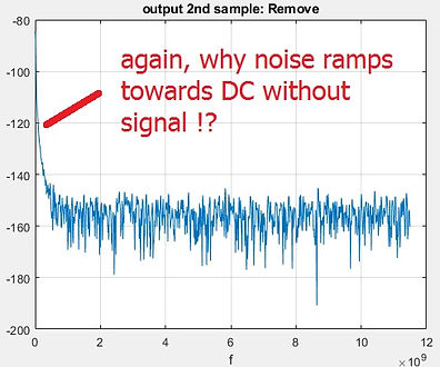
D3v(1,:)=[];

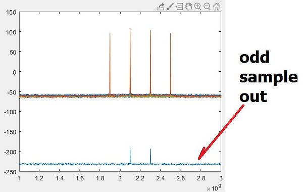
Video showing SA4 scope capturing output with input ramp, click on to watch [62]:

Again, for whatever reason. probably dsp.SpectrumAnalyzer limitation, the very first round produces a trace way below where it should be.

%% DATA PROCESSING 6

figure(23);

for k3=1:1:size(D3v,1)

plot(D3f,D3v(k3,:));

hold on

end

%% Odd sample out:

D3v(1,:)=[];

ramp2_dBm(1)=[]

hf24=figure(24);

for k3=1:1:size(D3v,1)

plot(D3f,D3v(k3,:));

% str1=input('prompt')

hold on

end

At this point, to be able to use findpeaks with MinPeakProminence and get all points needed to plot in-out power compression graphs, 3 things are needed:

Each line of D3v trace has to have 4 clear peaks.

These peaks prominence doesn't have to be above a certain constant value, they can be small, but all 4 peaks have to be above noise.

Define a variable peak prominence parameter to plug to Keep enough resolution to appreciate 1dB compression point and to calculate IP3

However input ramp is still too sharp, meaning that many early output traces contain 2F1-F2 and/or 2F2-F1 spurs below noise floor.

Literally documenting each ramp I have tried would unnecessarily extend this note.

So I have risen different input ramps until all 4 peaks could be caught by findpeaks with options SortStr NPeaks and MinPeakProminence.

As shown earlier a constant MinPeakProminence for findpeaks misses valid peaks [F1 F2 2F1-F2 2 F2-F1] and includes false peaks. To avoid this while using findpeaks with only MinPeakProminence and catch all only only relevant peaks, an increasing threshold for MinPeakProminence seems to do the job. L4 logs each distance from each trace max to a visually estimated -60dBm(W) noise floor, and L5 logs each distance between each trace max and the calculated root mean square noise floor

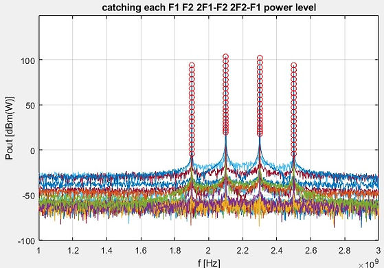
hf25=figure(25);

for k3=1:1:size(D3v,1)

plot(D3f,D3v(k3,:));ax25=gca;

hold on

end

grid on;xlabel('f [Hz]');ylabel('Pout [dBm(W)]')

title('catching each F1 F2 2F1-F2 2F2-F1 power level')

D4=NaN*ones(size(D3v,1),4)

for k=10:1:size(D3v,1)

[pks,locs]=findpeaks(D3v(k,:),'NPeaks',4, ...

'MinPeakProminence',L5(k)/1.8)

hold(ax25,'on')

plot(ax24,D3f(locs),pks,'ro')

D4(k,:)=pks

end

Let's assume that both 2F1-F2 and 2F2-F1 levels are needed, then both F1 F2 levels are also needed.

If the problem is on for instance just 2F1-F2 then only F1 or F2 is needed, whichever closer to 2F1-F2 .

To command plot one can either input 2 or 4 vectors, but for plot inputs to be consistent, same lengths are required.

I logged all data in NaN matrix D4 . What then happened was that for certain ramps the amount of NaN along each D4 column varied.

Now the right hand side shows D4 with ramp starting at

ramp2_dBm(1)

D4

on this particular input ramp the start level is high enough for all D4 columns to have same amount of NaN.

But I have come across, with test ramps not show, that detected peaks per trace may for from 0 to 4 taking all possible integer values. However, when the input ramp starts high enough then no NaN at all left behind in D4.

Input ramps starting too high cause measurements missing important data. or miss all the linear side of the Pout(Pin) graph, then the ramp starts where compression is already holding a1 and a3 graphs parallel.

So if the ramp starts low enough, as already mentioned, the amount of NaN per columns varies. Then one can manually 'trim' D4 or use the following:

The shortest vector sets the length for all others. Saying this is the same as saying that in D4 there shouldn't be any NaN left behind.

Removing any D4 line containing (one, more than one, scattered, bursted) NaN

L4=[];L5=[];

for k=1:1:size(D3v,1)

L4=[L4 max(D3v(k,:))-(-60)]

L5=[L5 max(D3v(k,:))-(-rms(D3v(k,:)))]

end

L20=zeros(size(D4,1),1);

if sum(sum(isnan(D4)))>0

for k=1:1:size(D4,1)

if sum(isnan(D4(k,:)))>0

L20(k)=sum(isnan(D4(k,:)));

end

[n1,n2]=find(L20>0);

D4(n1,:)=[]

ramp2_dBm(n1)=[]

=

1.724137931034483

D4 =

1.0e+02 *

NaN NaN NaN NaN

0.008825266193361 0.219361347021470 0.203922348473234 0.008159672102855

0.051867644191113 0.242364022706471 0.226970699503792 0.051307394343642

0.112235631549309 0.278249689861551 0.262818117497718 0.111633691001197

0.163944220678432 0.312569479869697 0.297130842754459 0.163357552518848

0.215652412246474 0.350221559901392 0.334789095920766 0.215064265312064

0.267386754696257 0.390998998680792 0.375560874560093 0.266798046798107

0.327713995387785 0.441921720388981 0.425597346626035 0.327679996422267

0.370111751410005 0.479543024125391 0.465559678090682 0.370919071119383

0.422558441461775 0.527586548548017 0.512148116795486 0.421972015215582

0.474287193121586 0.576287546705752 0.560847108540077 0.473701926976216

0.526001065403563 0.625903495473360 0.610463991848236 0.525417997498396

0.577713062545216 0.676175128559754 0.660705568533762 0.577184671889175

0.629413737902946 0.726892246823698 0.711435372833616 0.628948562980757

0.681252054451895 0.778061986138357 0.762373584691508 0.680553337867410

0.732871951654867 0.829230614581986 0.813764254497530 0.732383192150392

0.784471764016066 0.880513533543890 0.863339255092325 0.785008543859120

0.836337478193320 0.932185056777481 0.916717229058670 0.835799671563525

0.888107901638267 0.983816440080580 0.966161514492131 0.888842337938020

0.939799250659656 1.035415299263869 1.019976934399033 0.939212746063502

And here is where one can spot an important difference between the intermodulation polynomial model a_coeff and any real amplifier:

Real systems are power limited, therefore the only significant points towards IP3 calculation are the 1st 5 points on the left. The compression is modeled because both lines run parallel, but in real systems, with increasing input power, eventually, both blue and red lines end up flat on the right hand side.

D41=D4([1:6],2)

D42=D4([1:6],1)

D41 =

19.408441137601002

22.386018628352531

25.228332742389142

28.367275757259137

30.791354129775744

35.019604774894759

D42 =

-4.296594626408996

1.751516168463457

6.930863151457508

12.083378292850478

15.771778712805952

21.562360766958935

diff(D41)

diff(D42)

diff(D41) =

2.977577490751528

2.842314114036611

3.138943014869994

2.424078372516608

4.228250645119015

diff(D42) =

6.048110794872454

5.179346982994051

5.152515141392970

3.688400419955475

5.790582054152983

figure(26);ax26=gca

plot(ax26,ramp2_dBm,D4(:,2),'b*');

grid on

title('PinF1 vs PoutF1')

ax.DataAspectRatio=[1 1 1]

hold on

plot(ax26,ramp2_dBm,D4(:,1),'r*');

grid on

title('PinF1 vs Pout2F1-F2')

xlabel('Pin [dBm(W)]')

ylabel('Pout [dBm(W)]')

From this point to the end of this note, for the sake of brevity, it's an example only and because I considered important to elaborate on how to use dsp.SpectrumAnalyzer throughout the collection, this being 1st contact, I am skipping code in this note, and briefly mentioning key points:

y=p(x) for Pout(Pin) is a limited model

Rewording; the Pin(Pout) compression graph at the beginning of this example corresponds to a measurement on a real amplifier that has a linear in-out region, then a compression region, and as input power keeps increasing, a saturation region.

a_coeffs or any polynomial y=p(x) such as N=numel(a_coeffs);syms x;a_coeffs.*x.^[1:N] with x in y out, this is, merely taking into account the input signal amplitude to calculate y = a0 + a1*x + a2*x^2 + a3*x^3 +.. in order to shape output y on it's own cannot go any further than simulating only the right hand side of the opening Pout(Pin). If enough points in the right hand side of such graph, then it may be possible to calculate IP3 from slopes.

y=p(x) as defined in chapter 10 does not model the right side of the graph with flat responses.

Not taking into account power supply, the modelling of IP3 for any amplifier or for the case of any RF system, this is, not considering power consumption and the obvious limitations involved, is only a mathematical exercise that wishfully ignores the crucial fact that power consumption of any device should be included in its modelling, particularly when modelling effects like IP1dB IP2 IP3 and their real relations.

As obvious as it is, all power supplies are power limited: AC/AC AC/DC DC/AC or DC/DC, reaching the highest available power is what causes 1dB compression and eventual flat output for any fundamental, harmonic and spur, not y=p(x) behaviour. Including in power supplies safety devices to prevent reaching performance peak increases life time, reliability (MTFF MTBF ..) and the longer customers keep your reliable power supplies, the longer they will consider buying a power supply from a competitor.

Perhaps, also fold-back, cut-off, feed-back, feed-forward device may be additionally in place. The higher the power handled the more reasonable to include safety devices.

Also, such polynomial modelling cannot model, at all, the 1dB compression and eventual flat parallel curves on right hand side of opening Pout(Pin).

In a nutshell, when attempting to model a device built with transistors, it's a good idea to start the system modelling--- with transistor models, for all involved transistors, as well as any other involved electronic component. Active Devices in chapter 11, and Amplifiers in chapter 12. Chapter 10 is about important RF system measurements to obtain figures of merit so we can compare systems.

Need to measure close to noise floor

The smaller the signals used the higher the linearity obtained, therefore one can better interpolate both lines needed to calculated IP3

With ramp3_dBm and SA4 (code to generate ramp3_dBm and run SA4 attached script) among other results, I get these traces, closer to noise floor, and at the same time capturing all 4 relevant peaks

Another problem caused by over-simplified polynomial modelling: output power level samples of 2F1-F2 (or 2F2-F1) when input too low may have parabolic behaviour rendering any attempt to interpolate a line, to then calculate IP3 not valid.

Once all spurs combined, at least from the mathematical model, this system may even show

2 different input levels delivering same output power, something that has to be avoided when fitting the linear region of an amplifier in-out response.

The code on the right hand side of these lines, like the one next to 1st graph on this page, are reused cells for trial-and-error

One can ignore such spur output power parabolic behaviour if it's way below blue trace linear output.

These 2 graphs on the right hand side seem to intersect, they don't look parallel, at least from 10dBm in up, but one cannot tell whether this system has no noticeable intermodulation before reaching saturation, because if distance between traces, or it's already in compression/saturation, because neither the linear blue trace has slope 1:1 nor the spur red trace has slope 1:3.

This is caused by the particular choice a_coeff=[ .12 -.4 12 .5] (or a_coeff=[5 .4 12 .5]) used so far in this example, and in general for a_coeff with really low relative value of 3rd order product a3 compared to linear coefficient a1

a3/a1 << 1 keeps system generated spurs well below the linear response, but also pushes the spur in-out graph to the left of the opening Pout(Pin) graph.

I repeated it all with a_coeff=[1 1 1 1] and a_coeff=[20 1 10 1] and different ramps, with more steps.

With some further trial and error I realised that I was using way all too high input signal levels.

Similar a1 and a3 may be another problem for IP3 measurements, when combined with using off-range (too high or too low) input levels, because then the obtained curves are all already in saturation, without even noticing it.

Also, the condition a3 >> a1 is necessary to offset Pout3(Pin) to the right, away from Pout1(Pin) and the measurement Pout(Pin) in [dBm]/[dBm] to look like the opening graph of this example. Otherwise Pout3 starting too far to the left again is a misleading situation that prevents the measurement from a successful conclusion.

Eventually one gets the graph on the right hand side. The 'flat' points on the left side of the graph, for both traces, it's noise, cannot be used for IP3 calculation. And as already mentioned above, the far points on the right hand side with stiff slope, those are not model a real system, it's a limitation of the mathematical model. Checking 5 central points slopes:

p1=[8.27 -26.22]

p2=[17.93 .56]

% slope spur, red trace

(p2(2)-p1(2))/(p2(1)-p1(1))

% slope linear, blue trace

p3=[8.27 16.34]

p4=[17.93 26.51]

% slope linear

(p4(2)-p3(2))/(p4(1)-p3(1))

p1 =

8.270000000000000 -26.219999999999999

p2 =

17.930000000000000 0.560000000000000

=

2.772256728778467

p3 =

8.270000000000000 16.340000000000000

p4 =

17.930000000000000 26.510000000000002

=

1.052795031055901

Different input power ramps, the highlighted one produces Pout(Pin) with linear 1:1 and spur 1:3

N01=0; % [dBmW]

Pin_start2=10^((N01-30)/10)/1e4; % [W] start ramp

Pin_stop2=1e2/100; % [W] stop ramp

Pin_start2_dBm=10*log10(Pin_start2)+30; % [dBmW] start ramp

Pin_stop2_dBm=10*log10(Pin_stop2)+30; % stop ramp

N_ramp=30; % choose amount of levels, ramp resolution

ramp2_dBm=linspace(Pin_start2_dBm,Pin_stop2_dBm,N_ramp);

ramp2_W=10.^((ramp2_dBm-30)/10); % input power ramp [W]

ramp2_V_Z0=(ramp2_W*2*Z0).^.5;

hold(ax21,'on');stem(ax21,10*log10(ramp2_W)+30,'r', ...

'MarkerSize',10, ...

'MarkerEdgeColor','b', ...

'MarkerFaceColor',[.49 1 .63])

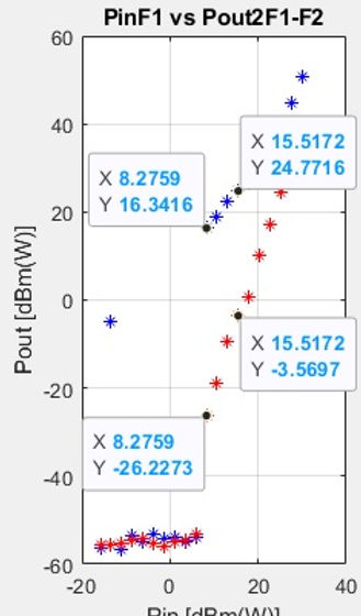
Removing the closest point to saturation

p1=[8.27 -26.22]

p2=[15.51 -3.57]

% slope spur, red trace

(p2(2)-p1(2))/(p2(1)-p1(1))

% and from the blue trace

p3=[8.27 16.34]

p4=[15.51 24.27]

% slope linear

(p4(2)-p3(2))/(p4(1)-p3(1))

p1 =

8.270000000000000 -26.219999999999999

p2 =

15.510000000000000 -3.570000000000000

=

3.128453038674033

p3 =

8.270000000000000 16.340000000000000

p4 =

15.510000000000000 24.270000000000000

=

1.095303867403315

m1=(p2(2)-p1(2))/(p2(1)-p1(1))

m2=(p4(2)-p3(2))/(p4(1)-p3(1))

c1=-p1(1)*m1+p1(2) % [dB] mind the gap [dBm]-[dBm]=[dB]

c2=-p3(1)*m2+p3(2) % [dB]

% IP3=[IIP3 OIP3]

IIP3_dB=(c2-c1)/(m1-m2)

OIP3_dB=m1*x0+c1

IIP3_dBm=IIP3_dB+30

OIP3_dBm=OIP3_dB+30

% check

m2*IIP3+c2=m1*IIP3+c1

m1 = 3.128453038674033

m2 = 1.095303867403315

c1 = -52.092306629834248

c2 = 7.281837016574586

IIP3_dB = 29.203043478260870

OIP3_dB = 39.268043478260871

IIP3_dBm = 59.203043478260867

OIP3_dBm = 69.268043478260864

=

logical

1

Note that slopes are in [dB]:[dB] and that when calculating constants c1 and c2, on subtracting [dBm] values, the result is always in [dB] therefore the intersection point has been obtained in dB(W)

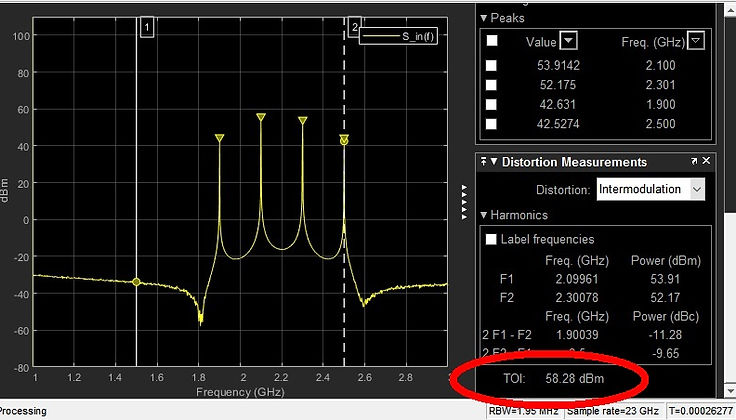
So the IP3 measurement delivered by dsp.SpectrumAnalyzer tagged TOI is IIP3_dBm that reads 58.28dBm.

For the particular a_coeff defined system there's a 1dB discrepancy with the manually obtained

[IIP3 OIP3]

command toi

The following RF measurements directly implemented with single command: sfdr sinad snr thd toi

f=[2.1 2.3]*1e9 % [Hz]

% Fs=10*max(f)

T=min(1./f)

dt=T/10 % time resolution

t=[0:dt:20*T]; % amount of cycles to simulate

Fs=1/dt

rng default % seed reset

x1 = sin(2*pi*f(1)*t1)+sin(2*pi*f(2)*t1);

xin = x1 + 0.01*x.^3 + 1e-2*randn(size(x));

[TOIdB,Pfund,Ffund,Pim3,Fim3] = toi(xin,Fs)

f =

1.0e+09 *

2.100000000000000 2.300000000000000

T = 4.347826086956522e-10

dt = 4.347826086956522e-11

Fs = 2.300000000000000e+10

TOIdB =

NaN

Pfund =

2.155729426319936 -39.198223498263474

Ffund =

1.0e+09 *

2.200447080143711 6.669434642112546

Pim3 =

NaN -47.558915805679767

Fim3 =

1.0e+10 *

NaN 1.124917630916316

I tried increasing the amplitude from the initial 0.01 but toi doesn't get to measure TOI returning NaN only .

Increased Fs 10 fold but toi returns NaN

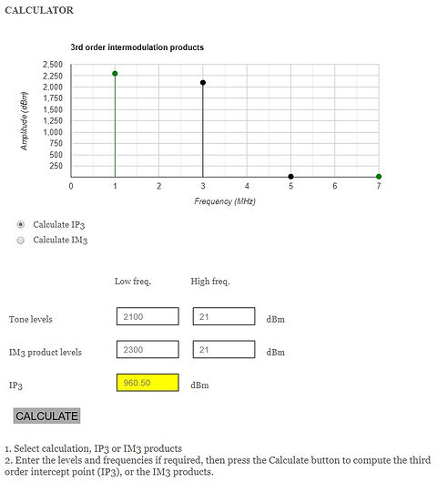
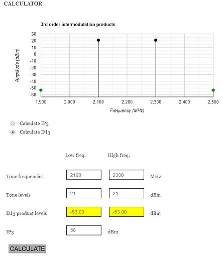
The IP3 online calculator in reference [61] doesn't work, neither for IP3 nor for IM3.

IP3 through cascaded blocks

Obtain OIP3'' knowing IIP3 then

G2_dB=-6

G2=10^(G2_dB/10)

IIP3_2_dBm=13

IIP3_3=10^((IIP3_2_dBm)/10)

OIP3_2_dBm=IIP3_2_dBm+G2_dB

OIP3_2=10^((OIP3_2_dBm-30)/10)

OIP3_1_dBm=22

OIP3_1=10^((OIP3_1_dBm-30)/10)

G2_dB =

-6

G2 =

0.251188643150958

IIP3_2_dBm =

13

IIP3_3 =

0.019952623149689

OIP3_2_dBm =

7

OIP3_2 =

0.005011872336273

OIP3_1_dBm =

22

OIP3_1 =

0.158489319246111

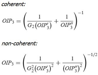
OIP3=(1/(G2*OIP3_1)+1/(OIP3_2))^-1

OIP3_dBm=10*log10(OIP3c)+30

OIP3c =

0.004451465972963

OIP3_dBm =

6.485030579747697

OIP3=(1/(G2^2*OIP3_1^2)+1/(OIP3_2)^2)^-.5

OIP3nc_dBm=10*log10(OIP3nc)+30

OIP3nc =

0.004972621871624

OIP3nc_dBm =

6.965854358437738

Note: As Mr Blattenberger points out in his website RF-café obtaining the overall IP3 through cascaded blocks may not be as simple as just plugging a formula while simply discerning whether used signals are coherent or not. Read [21] for more detail.

1dB compression point to IP3 relation

To calculate expected value before measurement of the Output 1dB compression point or OIP1 of single device with power gain G [dB] knowing the input 1 dB compression point or IIP1 [POZAR] pg513:

OIP1=IIP1+G-1

For amplifiers, although some low power amplifiers may be able to actually reach OIP3 or OIP2, IIP3 may not actually reach OPI3, therefore there's no need to actually reach the input-output power point, this point being where lines cross: 1dB compression, saturation, or any other undesired effect like overheating, safety cut-off, or worse took place.

One step further, one can 'advance' IP3 with just a 1dB compression measurement. A complete test; 1dB compression, IP3 ( or even IP2) may be carried out on a small sample of units, and then if the deviation of such measurements is acceptable, production line units may have IP3 calculated out of 1dB compression measurements only.

IP1dB=IIP3-9.6

For the detailed demonstration of IP1dB(IIP3) read [51]

In reference [23] there are 53 different real in-the-market amplifiers IP1dB compiled in a single table

In the attached MATLAB script for example 10.4 there is an additional cell not detailed in this note regarding What input level produces smallest discernible output level. This cell is open, beyond scope of example 10.4 but worth mentioning it and left for further work.

So far there's been no time to refine into local support flawless functions, that would have shortened the length of this note, but would have doubled the amount of time, already through budget roof.

References

pg26 on this note SA4 scope captured with OBS studio, video cropped for free with clideo.com, .mkv to .mpg4 free online translator uniconverter.

[CAER]

The Receiver Analysis and Design from a System Point of View, Thesis, J. Caeiro Nogueira, thesis 2013

https://fenix.tecnico.ulisboa.pt/downloadFile/395145531620/Dissertacao_MEE_54481.pdf

[JASP]

IP3 (3rd Order Intercept) by Bill Jasper, Presentation, Test Edge 011010 www.testedgeinc.com

[4]

Distortion Simulation with Simulink

https://uk.mathworks.com/help/dsp/examples/spectrum-analyzer-measurements.html?s_tid=srchtitle

[10]

The Use of Intermodulation Tables for Mixer Simulations, by D. Faria, L. Dunleavy, T. Svensen

https://www.microwavejournal.com/articles/3430-the-use-of-intermodulation-tables-for-mixer-simulations

[11]

.imt files figures 9-1, 9-2, pg 9.25

Advanced Design System 1.5, Circuit Components System Models

Agilent Tecnologies, February 2001

Two-Tone Envelope Analysis Using Real Signals

https://uk.mathworks.com/help/simrf/examples/two-tone-envelope-analysis-using-real-signals.html

[21]

RF Cafe - K.Blattenberger: RF Workbench cascaded modules Pin - Pout

https://www.rfcafe.com/business/software/rf-workbench/rfwb-system-screen.htm

[23]

RF Cafe - K.Blattenberger: cascaded IP1dB plus IP1dB, IP2 and IP3 from 53 datasheets

https://www.rfcafe.com/references/electrical/p1db.htm

[27]

Example of too few points in linear region, too many points in saturation.

with a_coeff=[20 1 10 1] and input ramp N_ramp=50;

ramp3_dBm=linspace(ramp2_dBm(1)+15,ramp2_dBm(5)+35,2*N_ramp); one now can see that the cubit spur is always going to eventually catch the linear region, but what system requires to operate far beyond saturation when one can have it operating just at the beginning of it, or Watts to waste anyway?

[51]

Accurate and Rapid Measurement of IP2 and IP3. May, 2002. By Kundert, S.Kenneth

http://www.designers-guide.org/Analysis/intercept-point.pdf

AVG RMS ratios for common waves, refresher

https://en.wikipedia.org/wiki/Root_mean_square

[61]

IP3 calculator at RF response doesn't seem to work correctly for 2.1 2.3 GHz input and 21dBm both input carriers, neither IP3 calculation nor IM3 product(s) calculation

IP3=960dBm is absurd

IM3 of -53dBm is way to low after what has been shown above.

http://rfresponse.com/calculators/ip3_2tone_chart.php?calc=IM3

[62]

When opening SA3 measurement video, while Chrome plays ok the video, in same folder as this note in .pdf, Edge claims file not found.

example 10.4

Since it's just a single value, with sign change, the expression matches [POZAR] pg516.

fint_ord 1st column contains spur frequencies, and 2nd column contains spurs intermodulation orders. Following spurs histogram over spur frequencies:

Doubling top spur frequency as number of histogram bins one achieves enough resolution, for a well defined spurs frequency histogram.

Spurs intermodulation orders histogram:

So, IP3 point Input Intermodulation Product 3 or IIP3 is defined by [IIP3 OIP3] and is the input power that would be needed for a given non-linear device to produce same amount of power out of the fundamental coefficient a1, and from the 3rd order coefficient a3 . When Pin=IIP3 then Pout=OIP3

​

​

​

​

​

​

​

​

​

​

​

Note that point IP2 can also be defined, out of IIP2 and OIP2 . However as [JASP] shows (next graph right hand side), for an increasing input signal OIP3 is typically reached before OIP2.

​

Intermodulation orders are proportional to Pin/Pout slope.

​

​

Heading 5

Spurs tend to show up around harmonics

figure(4);

​

These 2 graphs only show frequencies, the level is not significant. Input carrier amplitudes all set to 2, all outputs set to 1. The grouping of distortion spurs around harmonics is a bit clearer if the values of f are closer each other.

data_measurement

Sample, reading trace out of last (highest) input ramp level

​

​

Let's pull up input ramp 1st level from -60dBm up to -20dBm. Compressing the input ramp; same amount of steps, same stop input power, but higher ramp start input power.

Narrowing band to [1 3] GHz this way only 2F1-F2, 2F2-F1, F2, F1 show up:

​

Again, for whatever reason. probably dsp.SpectrumAnalyzer limitation, the very first round produces a trace way below where it should be.

Different input power ramps, the highlighted one produces Pout(Pin) with linear 1:1 and spur 1:3

Removing the closest point to saturation

​

The Use of Intermodulation Tables for Mixer Simulations, by D. Faria, L. Dunleavy, T. Svensen