ZIP with MATLAB scripts and note:
exercise 6.17
exercise 6.17 notes:


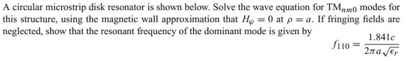
For this exercise, the solutions manual, like for 6.16, supplies one of the shortest answers, yet disc resonators are commonly used in modern circuits, not only for telecommunications but in test and measurement.
[LEON] quote: .. If a whispering gallery or a photonic crystal is free to oscillate, it acts as mechanical and optical resonator simultaneously ..
[HERM] quote: .. cavity optomechanics are ultra sensitive sensors for mass, chemical, biological sensing. VLSI with low-loss Si optomechanical microdisks (perform) 1e6 Q (while their) Brownian motion is resolved at few 100MHz in ambient air: this is the next generation of high-end sensors operating in vacuum, gas or liquid phase ..
While [POZAR] focuses on ring and disc planar resonators, there are other resonating structures commonly used, like: elliptic, rectangular, triangular patches, and (re-entrant) coaxial resonators only briefly mentioned once in chapter 8, and in reference [9] of same chapter, and planar patches with other shapes than circular. [BHAR] succinctly cover all the shapes mentioned, supplying curves obtained from measurements. The same way that I considered the parallel planes waveguide for an additional exercise, I also include additional MATLAB exercises for each additional resonating structure in 6.17.2 to 6.17.5.
Gallery whispering modes (WGM) are generated by fringing fields between dielectric resonator and any close enough transmission line(s).
In a different chapter than chapter 6 [POZAR] shows the following equivalent circuit, but no further comment is added regarding how to calculate L C R and N. Thanks to [BHAR] further down in this extended answer to exercise 6.17 and accurate explanation is supplied regarding the tank circuit approximation of a close enough dielectric object to transmission line with characteristic impedance Z0.

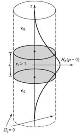
[POZAR] next approximation is to assume fields 'reasonably' confined within the dielectric.
[POZAR] doesn't mention whether the disc is metallic or dielectric.
One of the key applications of resonating dielectric discs is to sharpen Q of oscillators. A little compact chunk of dielectric placed on the right spot, close enough, far enough, it has a far sharper frequency filtering effect to for instance reject noise and interference on antenna, than a meticulously calculated 20 stages Chevyshev band pass filter.
[POZAR] neither has alphabetical index entry for 'DRO' nor for 'Dielectric Resonator Oscillator'. Yet in example 13.4 (pages 618 to 622), key calculations for DRO design are included.
The logic question then is: what happened to the TE01d mode strongly depending upon fringing fields, [POZAR]
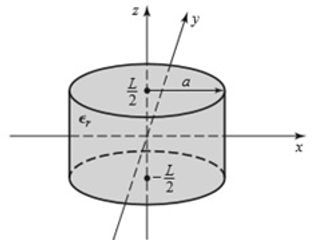
[POZAR] simplifies imposing magnetic wall at r=a which may be reasonable because the DRO may be sandwiched between metal plates, but then the calculation of the resonant frequencies is reduced to solving the equation on the right hand side:
However, same [POZAR] admits that this approximation, that ignores fringing fields (in [NBush] called 'bifringent') which are precisely the fields enabling the resonator to resonate, may suffer over 10% error, and [POZAR] again, closes the DRO example with, [POZAR] quote
The resonator operates in TE01d mode, and couples to the fringing magnetic field of the microstrip line.

usually not accurate enough for practical purposes
The next logic question being: What is the point of calculating oversimplified DRO parameters if it may be the case that obtained values are too coarse?
Given the wide scope of [POZAR] and how light goes on such device, I decided to build some background before getting on scripts to help design circuits like such resonators. Following, a sampled version of the note attachments to this text, read all attachment here.
[BHuff] refraction study at particle level page 188 shows that electromagnetic resonance takes place where following coefficients peak.
-
incident Electric field parallel to XZ plane,
-
incident Electric field perpendicular to XZ plane
b and a are normalised wave scattering parameters applied to a potpourri of spherical particles, a and b related to the fields of interest the following way:
small a and b not to be confused with capital A and B
And from [BHuff] the equations to solve, in order to find resonant wavelengths [TRGSN] or frequencies is for wave E || XZ plane
and E ^ XZ plane :


However [NBusch] simplifies the calculation of resonant frequencies to just resolving the E || XZ plane equation:

to calculate resonant frequencies (obviously before validating through measurement).
QL is resonance out of left-handed circularly polarised wave
QR is resonance out of right-handed circularly polarised wave
Mind the gap; [BHuff] variable m is [NBush] n and vice versa.
As example [NBusch] shows that for dielectric with diffraction index n=1.59, normalised radius r=1 (no units) and [m l ]=[18 1] then the normalised resonant frequency is f0_18_1=Re(w0)/(2*pi)=2.065
m: azimuthal order of resonance (how many 'peaks' has the crown) and l is radial order, the amount of 'crowns' that is same as resonance frequency order.
with resonance quality factor:
Q0_18_1=-Re(w0)/(2*Im(w0))=829.5
check: w0=12.9747 Im(w0)=.00782
harminv
meep
Simpetus: MEEP MPB SCUFF-EM
https://www.youtube.com/watch?v=_c3PT_rzmMM
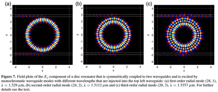
[BHuff] figure 7: 3 simulations show how electromagnetic average energy is distributed over a resonant dielectric disc located between 2 parallel microstrip transmission lines, for 3 different [m l ] values. Only case 3 allows wave forward along the top transmission line.
Resonance takes place because a significant part of the incident wave (or all of it) on the dielectric ring or disk is trapped inside the dielectric through multiple reflections.
On the right hand side [BHuff] page 167, if the ray is not tangent enough there's significant outwards refraction. IF too close to tangent line, the wave may not get in.

From [TRGSN] at certain frequencies the incident wave remains confined inside the dielectric disk remaining confined following a polygonal path
R is confined ray, the section of straight path between 2 consecutive internal bouncing points, aka polygonal whispering gallery ray.
R is related to resonant wavelength with the expression in the right hand side, n=er^.5 with n the refractive index, er relative permittivity.
Resonating waves are trapped because the wave energy remains on a constant radius, showing periodic peaks and valleys along varying angle.
N is the azimuthal order; the amount of spots the confined wave hits the edge of the dielectric disk.
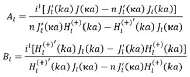
[TRGSN] uses same notation as [BHuff] for forward/return field coefficients A_L and B_L