exercise 6.16
pozar_06_ex_16_DE_simulation.zip

pozar_06_exercise_16_support_docs.zip
exercise 6.16 notes:

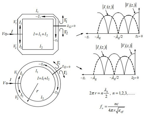
Resonance happens when a signal finds either Open Circuit or Short Circuit at a multiples of lambda/2.
This is not about a wireless radio wave hitting this ring and then finding out how much signal is reflected.
Although not shown, neither in [POZAR] nor in the solutions manual, but there has to be a signal source somewhere 'connected' to the ring resonator, on one or 2 points of the ring. This resonators are used as sensors and the generator coupling(s) is actually a narrow enough gap(s) that behave(s) as capacitor(s).
The solutions manual only supplies one half of the answer.
As [LNG] Lung-Hwa mentions in page 9 of his thesis, there's at least one literature error (referenced in [LNG]), and [VIT] also points the same, that it's not only at 2*pi*R= Lring = n* lambda when a ring resonator may resonate, but also at pi*R = Lring/2 = n* lambda/2 depending upon 2 or 1 source points respectively.

[LNG]
Analysis modelling and simulation of ring resonators and their applications to filters and oscillators, May 2004, thesis by Lung-Hwa Hsieh at Texas A&M University, https://core.ac.uk/download/pdf/4268464.pdf copy supplied attached to this note.
[VIT]
Review of different ring resonator coupling methods, by A.Vitas Athens University.
https://pdfs.semanticscholar.org/73ac/e049d10f989adc72b0b158c0e0a17e1a7618.pdf
[BOG]
Planar Microstrip Ring Resonators for Microwave-Based Gas Sensing: Design Aspects and Initial Transducers for Humidity and Ammonia Sensing. September 2017, by Bogner et al. IEEE Sensors
single feed point, from [LNG] 2 feed points [BOG] and [LNG]

I have modified example 4.b from [ED]. [ED] authors split scripts into many different small modules. If one needs the original scripts, the authors of reference [ED] send by email to purchasers of their book the entire collection of MATLAB scripts.
This note is accompanied by 2 ZIP folders, one with a basic working simulation of a single feed ring resonator: pozar_06_exercise_16_ED_sim.zip and pozar_06_exercise_16_support_docs.zip .
To play, modify as you wish, and/or improve the simulation, put all files from 1st .zip into same folder and run fdtd_solve.m
pozar_06_ex_16_DE_simulation.zip
microscrip TL loaded with resistor.fig
V_source vs V_sample.fig
capture_sampled_currents.m
capture_sampled_electric_fields.m
capture_sampled_magnetic_fields.m
capture_sampled_voltages.m
create_linear_index_list.m
create_PEC_plates.m
define_geometry.m
define_output_parameters.m
define_problem_space_parameters.m
define_sources_and_lumped_elements.m
display_3D_geometry.m
display_animation.m
display_material_mesh.m
display_material_mesh_gui.m
display_objects_mesh_in_animation.m
display_problem_space.m
display_sampled_parameters.m
display_transient_parameters.m
fdtd_solve.m
initialize_animation_parameters.m
initialize_boundary_conditions.m
initialize_capacitor_updating_coefficients.m
initialize_current_source_updating_coefficients.m
initialize_diode_updating_coefficients.m
initialize_display_parameters.m
initialize_fdtd_material_grid.m
calculate_material_component_values.m
initialize_inductor_updating_coefficients.m
initialize_output_parameters.m
initialize_resistor_updating_coefficients.m
initialize_sources_and_lumped_elements.m
initialize_updating_coefficients.m
initialize_voltage_source_updating_coefficients.m
initialize_waveforms.m
Vsource_vs_Vsample_single_graph.m
main_define_output_parameters.m
calculate_domain_size.m
object_drawing_functions.m
plot_e_xy.m
plot_e_yz.m
plot_e_zx.m
plot_h_xy.m
plot_h_yz.m
plot_h_zx.m
post_process_and_display_results.m
run_fdtd_time_marching_loop.m
set_color_axis_scaling.m
solve_diode_equation.m
update_current_sources.m
update_diodes.m
update_electric_fields.m
update_inductors.m
update_magnetic_fields.m
update_voltage_sources.m
initialize_fdtd_parameters_and_arrays.m
pozar_06_exercise_16_support_docs.zip
BOG ring resonator sensor for NH3 detection - Bogner Steiner.pdf
LNG Hsieh thesis on ring resonators - TX Uni.pdf
pozar_06_exercise_16.pdf
pozar_06_exercise_16_question.jpg
VIT ring resonators review - A Vitas et al.pdf
I know, it's just an insignificant ring resonator, so why so many .m files? First, the 'so many' is relative to 'as many' as required, whatever it takes, to solve the problem.
Also [ED] has a template that, step by step, it's revealed along their book. Yet they started their MATLAB list of scripts with a jamming 1D example, so slow that probably half readers were at that early reading point put off, for ever, to tough again [ED] book or even learn MATLAB, both mistakes because [ED] is a really good book and MATLAB is increasingly taking over tools at solving problems where some years ago it was only one of many ancillary post processing data 'shovel'. Many of the .m files are really small, one only contains a call to another support file.
where Hsieh [LNG] writes mode 1, it should be: mode 2 for 1 port, mode 1 for 2 ports
mode 1 for 1 port would look like this
I have modified [ED] Transmission Line + Resistor example 4.a .
In define_geometry.m one can build any 3D geometry with MATLAB.
For instance, the following code lines define a '4 sides' ring:


% dimension basic block
Lx=20e-3
Ly=2e-3
Lz = 4e-3 % substrate thickness
%%% signal
% define PEC plate 1 : signal : v1 [0 0] -> v2 [20 0]
bricks(1).min_x = 0; bricks(1).min_y = 0; bricks(1).min_z = Lz;
bricks(1).max_x = Lx; bricks(1).max_y = Ly; bricks(1).max_z = Lz;
bricks(1).material_type = 2;
% define PEC plate 2 : signal : v2 [20 0] -> v3 [20 20]
bricks(2).min_x = Lx-Ly; bricks(2).min_y = 0; bricks(2).min_z = Lz;
bricks(2).max_x = Lx; bricks(2).max_y = Lx; bricks(2).max_z = Lz;
bricks(2).material_type = 2;
% define PEC plate 3 : signal : v3 [20 20] -> v4 [0 20]
bricks(3).min_x = 0; bricks(3).min_y = Lx-Ly; bricks(3).min_z = Lz;
bricks(3).max_x = Lx; bricks(3).max_y = Lx; bricks(3).max_z = Lz;
bricks(3).material_type = 2;
% define PEC plate 4 : signal : v4 [0 20] back to vv1 [0 0]
bricks(4).min_x = 0; bricks(4).min_y = 0; bricks(4).min_z = Lz;
bricks(4).max_x = Ly; bricks(4).max_y = Lx; bricks(4).max_z = Lz;
bricks(4).material_type = 2;
%%%%%%
% ground
% define PEC plate 1 : ground : v1 [0 0] -> v2 [20 0]
bricks(5).min_x = 0; bricks(5).min_y = 0; bricks(5).min_z = 0;
bricks(5).max_x = Lx; bricks(5).max_y = Ly; bricks(5).max_z = 0;
bricks(5).material_type = 2;
% define PEC plate 2 : ground : v2 [20 0] -> v3 [20 20]
bricks(6).min_x = Lx-Ly; bricks(6).min_y = 0; bricks(6).min_z = 0;
bricks(6).max_x = Lx; bricks(6).max_y = Lx; bricks(6).max_z = 0;
bricks(6).material_type = 2;
% % define PEC plate 3 : ground : v3 [20 20] -> v4 [0 20]
bricks(7).min_x = 0; bricks(7).min_y = Lx-Ly; bricks(7).min_z = 0;
bricks(7).max_x = Lx; bricks(7).max_y = Lx; bricks(7).max_z = 0;
bricks(7).material_type = 2;
% define PEC plate 4 : ground : v4 [0 20] back to vv1 [0 0]
bricks(8).min_x = 0; bricks(8).min_y = 0; bricks(8).min_z = 0;
bricks(8).max_x = Ly; bricks(8).max_y = Lx; bricks(8).max_z = 0;
bricks(8).material_type = 2;
define this structure :

to add 2nd probe, in define_output_parameters.m
% PROBE 1
% define sampled voltages
sampled_voltages(1).min_x = 5.0e-3; sampled_voltages(1).min_y = 0; sampled_voltages(1).min_z = 0;
sampled_voltages(1).max_x = 5.0e-3; sampled_voltages(1).max_y = 2.0e-3; sampled_voltages(1).max_z = 4.0e-3;
sampled_voltages(1).direction = 'zp';
sampled_voltages(1).display_plot = true;
% define sampled currents
sampled_currents(1).min_x = 5.0e-3; sampled_currents(1).min_y = 0; sampled_currents(1).min_z = 4.0e-3;
sampled_currents(1).max_x = 5.0e-3; sampled_currents(1).max_y = 2.0e-3; sampled_currents(1).max_z = 4.0e-3;
sampled_currents(1).direction = 'xp';
sampled_currents(1).display_plot = true;
% PROBE 2
% define sampled voltages
sampled_voltages(2).min_x = Lx-Ly; sampled_voltages(2).min_y = Lx-Ly; sampled_voltages(2).min_z = 0;
sampled_voltages(2).max_x = Lx; sampled_voltages(2).max_y = Lx-Ly; sampled_voltages(2).max_z = Lz;
sampled_voltages(2).direction = 'zp';
sampled_voltages(2).display_plot = true;
% define sampled currents
sampled_currents(2).min_x = Lx-Ly; sampled_currents(2).min_y = Lx-Ly; sampled_currents(2).min_z = Lz;
sampled_currents(2).max_x = Lx; sampled_currents(2).max_y = Lx-Ly; sampled_currents(2).max_z = Lz;
sampled_currents(2).direction = 'xp';
sampled_currents(2).display_plot = true;
Add another figure to overlap input output measurements that [ED] keeps showing, continuous dashed lines for input output, but no code supplied to that effect.
In postprocess_display_results.m add something like this:
Don't worry about the resistor, it's set to very high impedance. In define_sources_and_lumped_elements.m
Change frequency in define_sources_and_lumped_elements.m
v1=voltage_sources(1).waveform(1:time_step);
figure; plot(time(1:time_step)*1e9,v1,'b-','linewidth',1.5);grid on
title('V in out');xlabel('t[ns]')
hold all
v2=sampled_voltages(1).sampled_value;
plot(time(1:time_step)*1e9,v2,'r--','linewidth',1.5)
% display probe 2 voltage measurement
figure; plot(time(1:time_step)*1e9,v1,'b-','linewidth',1.5);grid on
title('V in out');xlabel('t[ns]')
hold all
v2=sampled_voltages(2).sampled_value;
plot(time(1:time_step)*1e9,v2,'r--','linewidth',1.5)
% resistors
% direction: 'x', 'y', or 'z'
% resistance : ohms, magitude : volts
resistors(1).min_x = 7.0e-3;
resistors(1).min_y = 0;
resistors(1).min_z = 0;
resistors(1).max_x = 8.0e-3;
resistors(1).max_y = 2.0e-3;
resistors(1).max_z = 4.0e-3;
resistors(1).direction = 'z';
resistors(1).resistance = 5000000;
waveforms.sinusoidal(1).frequency =
waveforms.sinusoidal(2).frequency =

3GHz is close to the double feed 1st mode resonating frequency of ring with length Lring=4*Lx with Lx=.02
At f0= c0/(4*Lx) with 2 feeds (although there's only one) the probes show the following
waveforms.sinusoidal(2).frequency = c0/(4*Lx);
waveforms.sinusoidal(1).frequency = c0/(4*Lx);

and at, as [LNG] well spotted, half ring length is resonant wavelength for single feed,
waveforms.sinusoidal(2).frequency = c0/(2*4*Lx);
waveforms. sinusoidal(1).frequency = c0/(2*4*Lx);
as expected a peak of amplitude on the furthest far away point of the ring from the feed, as Lung shows


